 |
This section describes additional data files available from the FUSE
archive that can be used to support the analysis and understanding of FUSE data. Some of these
data files were used by CalFUSE to produce the calibrated data products,
and others contain information which can be used to verify the pointing,
performance, or status of the satellite or instrument during data acquisition.
This chapter contains information potentially useful to the "Advanced" and "Intermediate" users. However its contents are not of immediate relevance to the "Casual" user. The file naming convention used throughout this chapter has been described in Section 4.1.2.
Two nearly identical Fine Error Sensor (FES) cameras were available on FUSE. FES A was prime for most of the mission, and observed the LiF1A FPA. FES B became prime on 12 July 2005 and was used for the remainder of the mission. It observed the LiF2A FPA. Because the two cameras are on opposite sides of the instrument, the astronomical orientation in the images will appear flipped with respect to each other. Referring to the guide star plots for a given observation will provide confirmation of the expected astronomical orientation and star field expected for a given target (see Section 5.6 below).
An image from the active FES camera was routinely acquired at the end of an
observation to allow verification of the pointing of the spacecraft. Depending
on the phase 2 observing proposal instructions provided by the user,
this FES image would be obtained
either with the target in the observing aperture or at the reference point
(55.18 "
from the HIRS aperture, displaced towards the center of the FES
field of view; see Fig. 2.2). By convention, this exposure always has exposure ID 701,
which is used to distinguish this image from acquisition images.
Other FES images were obtained throughout each observation during the initial guide
star acquisition and subsequent reacquisitions (usually after the target
had been occulted). These images are
also stored and are available to the observer, although the target may be offset or
even absent in these images (e.g. if the target had drifted during occultation,
etc.). These images have observation IDs
and exposure IDs identical to the those used for the associated (usually
directly following) FUV exposure.
After the gyroless target acquisition software was
loaded, it was routine to obtain multiple images during each acquisition, and also during
reacquisitions resulting from loss of pointing stability. Each of the resulting images is stored in a
separate extension in the FITS file.
For most users, the final "end-of-observation" FES image (exposure 701) will be the
only image of interest.
The active image area of the FES CCD images was
512 × 512 pixels,
with pixel size of 2.55″.
An unbinned image has 8 rows and 8 columns
of overscan, resulting in a
520 × 520
raw image. These are the
sizes for the FES images obtained at the end of each exposure. Binned
images also have binned overscan, so a
2 × 2 binned image will have
size
260 × 260 pixels.
After the
gyroless target acquisition software was loaded, 4 × 4 binned images
were routinely obtained during acquisitions in addition to 2 × binned
images, resulting in a size of 130 × 130 pixels.
The raw data (*fesfraw.fit files) are stored as unsigned integers in
FITS extensions. The
calibrated FES images (*fesfcal.fit images) are processed by stripping
the overscan areas, and subtracting the bias level. Distortion maps of each FES camera
were made and used onboard by the guidance system, but distortion corrections
were not part of the calibration pipeline process, and so the calibrated
images have not had this correction applied. Distortions are generally
small, however. The calibrated
data values are 4-byte floating-point numbers.
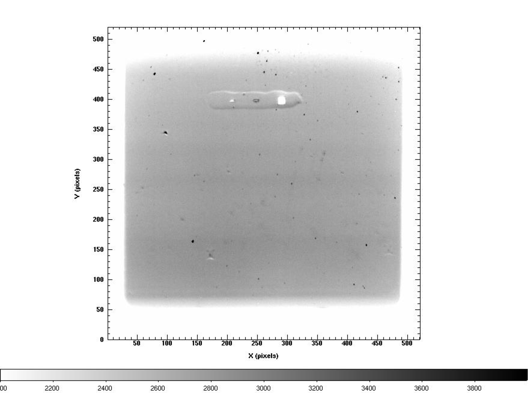
Figure 5.1 shows an example of a
512 × 512 FES A image.
Note that the apertures are near the top of the image along the line
defined by
Y_FES = 399 (see Table 5.2. Once again, users
will find the guide star plots (see Section 5.6) useful for
verifying the astronomical orientation expected for a given observation.
The contents of an FES file are listed in Table 5.1 and the locations of the apertures in pixels coordinates are listed in Table 5.2 for both FES A and B at the nominal LiF FPA positions. Details of the distortion corrections and the conversion of FES pixel coordinates to sky coordinates are provided in Section 8 of the FUSE Instrument Handbook (2009).
|
| FITS Extension | Format | Description |
|---|---|---|
| HDU 1: Empty (Header only) | ||
| HDU 2: FES Imagea | ||
| IMAGE | SHORT | COUNTS |
| a Image size can be either 520 × 520, 260 × 260 or 130 × 130. | ||
| FES A | FES B | |||
|---|---|---|---|---|
| Slit | X | Y | X | Y |
| MDRS | 207 | 399 | 292 | 426 |
| HIRS | 247 | 399 | 252 | 425 |
| LWRS | 289 | 399 | 209 | 425 |
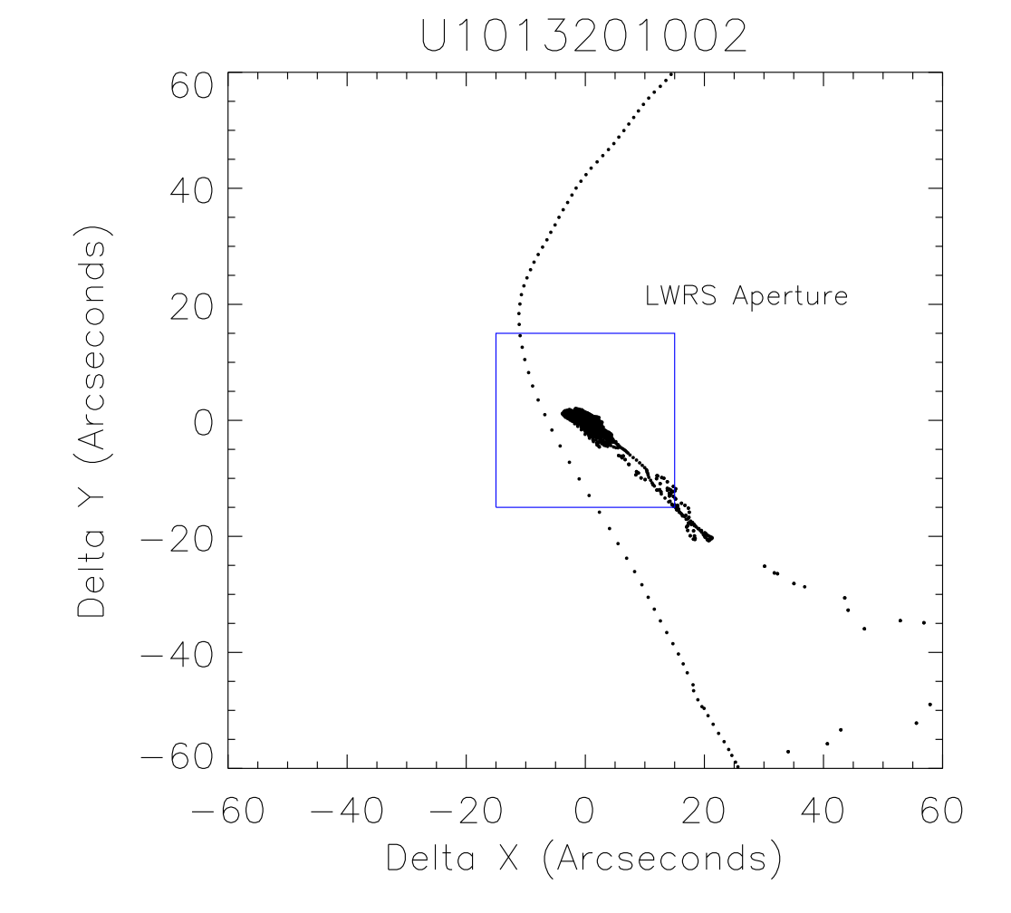
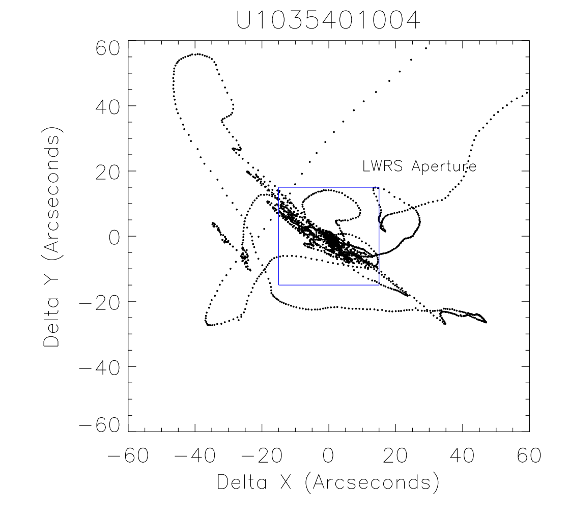
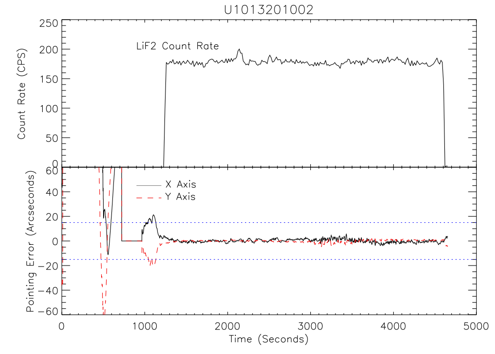
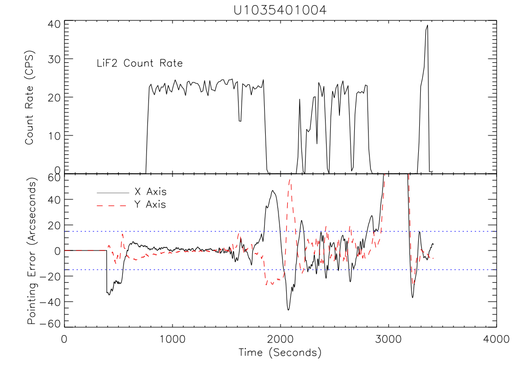
Jitter Files (*jitrf.fit): At launch, the pointing stability
of FUSE was approximately
0.3″ in the science X and Y axes. Since this is considerably
smaller than the instrumental PSF, guiding performance was not an issue for observing.
However, as the mission progressed, problems with the Attitude Control System
(see Table 2.3) required magnetic torquer bars and magnetometers be used
to help control the pointing. The ability of the torquer bars to stabilize the spacecraft depended on
their orientation relative to the direction of the instantaneous Earth's magnetic field,
which was a function of orbital position. As a result,
large, rapid pointing deviations caused by temporary loss of pointing control could
cause the target to move about in the aperture or leave it completely for
part of an exposure. Figure 5.2 and 5.3 show examples of pointing
performance and its effects on the FUSE count rates.
| 
|
| 
|
The orientation of the telescope is described by a four-element quaternion.
The spacecraft produced two sets of pointing estimates. The
first was derived from the measured positions of two to six guide stars;
these are referred to as the FPD (for Fine Pointing Data) quaternions. The
second combines guide-star data with data from the gyroscopes and magnetometers.
Since they are generated by the onboard ACS (Attitude Control System)
computer, they are referred to as the ACS quaternions, although the former
are not always available. The guide stars are
generally more accurate than the gyroscopes and magnetometers, so the FPD
quaternions are generally more accurate than the ACS estimates. The commanded
quaternions for the target can be found from the telemetry stream or computed
from the RA and DEC in the FITS file header (see the
Instrument Handbook 2009,
for more details).
The jitter data files contain time-resolved data of the spacecraft pointing relative to the commanded pointing and are used by CalFUSE to correct for these effects. These data are derived from the housekeeping files. This file is a binary table (see Table 5.3) with 1 s time resolution, and contains the following four variables:
| FITS Extension | Format | Description |
|---|---|---|
| HDU 1:Empty (Header only) | ||
| HDU 2: Pointing Data (binary extension) | ||
| TIME | FLOAT | (seconds) |
| DX | FLOAT | Δ X position (arcsec) |
| DY | FLOAT | Δ Y position (arcsec) |
| TRKFLG | SHORT | Quality Flag |
| a Sampled once per second, and dimension set length of the exposure. | ||
Housekeeping Files (*hskpf.fit): In addition to providing
inputs for the calculation of jitter parameters and the evaluation of
pointing quality, the housekeeping files contain time-resolved engineering data used by CalFUSE
to correct science data for instrument or pointing problems during exposures.
The housekeeping files are produced by the FUSE OPUS HSKP process from
files of telemetry extracted from the FUSE telemetry database for each
science exposure (TTAG or HIST). The time period included in the telemetry
files begins 0.5-1.0 minutes before the science exposure and ends 1.0
minute after the science exposure ends, to ensure that all the necessary
information is included.
A brief description of the contents of housekeeping
file is given in Appendix D. The data are stored in a binary table. Array
names are derived from the telemetry parameter in the engineering telemetry
database. Telemetry values are placed in time bins according to the time
at which the parameter is reported by the spacecraft (in units of MJD
days). The update rates are given in
Table 5.4. Due to lack of precision, the bins are not precisely
integer seconds in length.
Nominal update rates range from once per second to once every 16 s depending on the
telemetry item, but different telemetry modes sometimes changed the rates.
The time duration (in seconds) of the telemetry
included in the file can be obtained from the value of NAXIS2 in the
HDU2 header.
Any parameter not reported in a given second is given the value of "−1" in
the housekeeping file. Occasionally, parameters are reported twice in a
second, in which case only the final value reported during that second is placed
into the housekeeping file.
Each type of parameter is checked for telemetry gaps based on its nominal
update period. Gaps are reported in the trailer file for each exposure.
| Parameter(s) | Period (sec) |
|---|---|
| AATTMODE | 5 |
| ATTQECI2BDY | 2 (rarely, 0.2 s) |
| I_FPD | 1a |
| CENTROID | 1a |
| any I_ not already covered | 16 |
| AQECI2BDYCMD | 3 (rarely, 1 s) |
| a Only updated when using guide stars. The integration time for faint guide stars is 1.4 s. | |
The engineering snapshot data described in this section are somewhat of an anachronism,
and are included primarily for completeness. The contents of all of these
files are similar (see Appendix E), and provide a sampling of the
satellite and detector telemetry at the time they were recorded.
Engineering telemetry and science data for FUSE were stored and
downlinked in different data streams. Certain engineering parameters from
the instrument, such as detector temperatures and voltages, were identified
before launch as potentially being necessary for processing and calibrating the science
data. To capture that information, engineering
snapshots were taken at the beginning of an exposure and every 5 minutes
thereafter, with a final one taken at the end. These data were transmitted
in the science telemetry stream. The time of the first and
last snapshot were used by OPUS to define the exposure start and stop time for the science data. Other
snapshot data were used by OPUS to populate parameters in the FITS header
for the exposure files. A subset of these data for the detector are
available in the engineering snapshot files.
As the mission progressed, it was discovered that more engineering
telemetry at higher sampling rates were needed for CalFUSE to properly
process the science data. As a result, the housekeeping files, described
in previous sections, were created from direct extractions from the engineering archive,
and they were used to provide the necessary supplemental data.
Engineering snapshot data filenames have syntax as shown below, where *snapf* is used for standard engineering snapshot files, *snpaf* is used for engineering snapshots associated with FES A, and *snpbf* is used for engineering snapshots associated with FES B. Example file names are D0640301001snapf.fit and D0640301001snpaf.fit.
One Association Table is generated and used by OPUS (see Section 3.2)
for each observation. The file is formed of two HDUs as shown in Table 5.5.
HDU1 is a header containing basic information about the proposal, the observation and the target.
HDU2 is a list of which files were associated with a given observation, their type and whether
the files were found. An example is D0640301000asnf.fit with a generic naming as follows.
| FITS Extension | Format | Description |
|---|---|---|
| HDU 1: Empty (Header only) | ||
| HDU 2: Exposure association information | ||
| MEMNAME | STRING | Exposure names |
| MEMTYPE | STRING | EXPOSURE |
| MEMPRSNT | STRING | T/F |
This section describes the graphical timeline plots of the Mission Planning Schedules (MPS). These plots provide an overview of activities and orbital events throughout the mission and may be useful for placing observations and exposures into context. These plots indicate the PLANNED sequence of activities, and do not reflect any anomalies that might have occurred during actual execution of the observations. (For that see the daily count rate plots discussed in Section 5.7.) The MPS plots were generated for use by the Science Operations staff, and some of the items shown are specific to their needs. However, many of the parameters may be of interest to those who want to use the data as well. Hence, MPS plots have been added to the available FUSE products at MAST as part of the FUSE mission close-out activities.
The files are named according to the starting date of the MPS and FUSE orbit number (since launch). For instance: mps_2002_318_17869.001.pdf corresponds to an MPS which begins on year 2002, day 318 (e.g., November 14) and FUSE orbit number 17,869.
Figure 5.4 provides an example of a one day MPS timeline plot.
The plots are PDF files, usually with a day per page, and Day/Universal
Time as the abscissa. Each calendar day is broken into two panels, each covering 12 hours.
During nominal operations, MPSs typically covered a
one-week period, although actual times could be longer or shorter, depending
on conditions at the time of planning. Later MPSs were usually multi-day schedules (up to 2 weeks in
length) unless a re-delivery or re-plan had taken place.
MPS plots relevant to each observation can be accessed from the MAST preview pages.
The link connects to the PDF file of the MPS containing the observation, but the
user will need to page through the MPS file to find the specific observation of
interest. Inspection of these plots allows the user to assess many aspects of the
observation, including (for example) whether SAA passages impacted the scheduling,
whether low or grazing earth limb angles may have caused unusual airglow in the
observation, and which observations were scheduled before or after the observation
of interest.
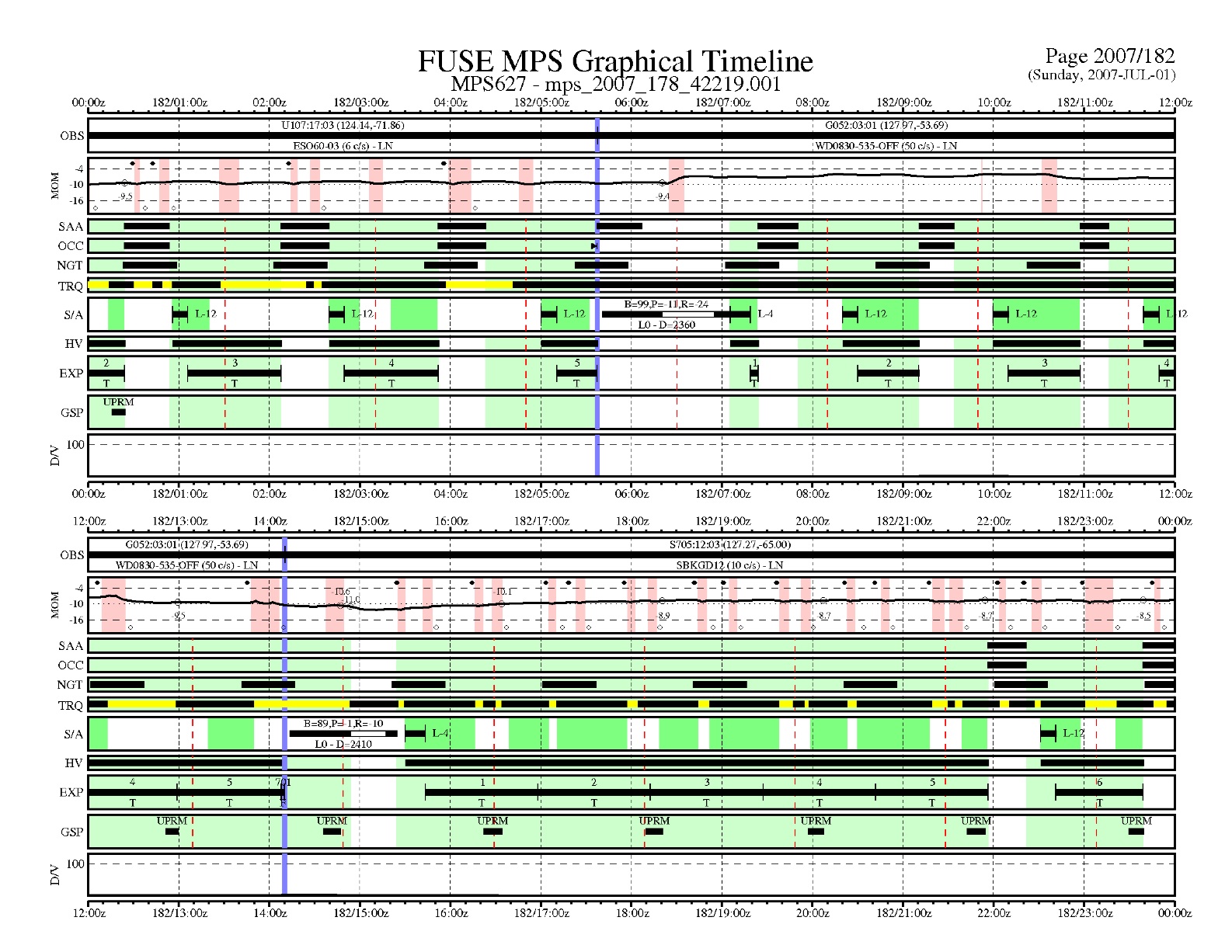 |
A variety of parameters are shown in sub-panels along the ordinate of these plots. The parameters plotted on these plots changed during the course of the mission, reflecting changing operational constraints and the evolution of mission planning tools. The following is a complete list of all possible parameters (and explanations) that appear in various MPS timeline plots.
Small slews and acquisitions. Acquisitions are labeled with the aperture (L - low, M - medium, H - high, R - reference point) and the acq_case. The acq_cases are:
Also shown on some of the plots are colored regions, and vertical lines. These indicate:
Table 5.6 lists the time ranges when different combinations of parameters were plotted on MPS plots.
| Datesa | MPS Nos. | Parameters |
|---|---|---|
| 1999-203 -- 2000-309 | 001-222 | RAM, LIMB, OBS, SLEW, ACQ, EXP, SAA, OCC, TMX, GSP |
| 2000-313 -- 2001-179 | 223-282 | OBS, LIMB, SAA, OCC, NGT, SLW, ACQ, EXP, GSP, DV |
| 2001-181 -- 2002-115 | 283-344 | OBS, LIMB, SAA, OCC, NGT, S/A, HV, EXP, GSP, DV |
| 2002-120 -- 2005-250 | 345-533 | OBS, LIMB, SAA, OCC, NGT, TRQ, S/A, HV, EXP, GSP, DV |
| 2005-264 -- 2007-262 | 534-633 | OBS, MOM, SAA, OCC, NGT, TRQ, S/A, HV, EXP, GSP, DV |
| a The format is: YYYY-DDD -- YYYY:DDD | ||
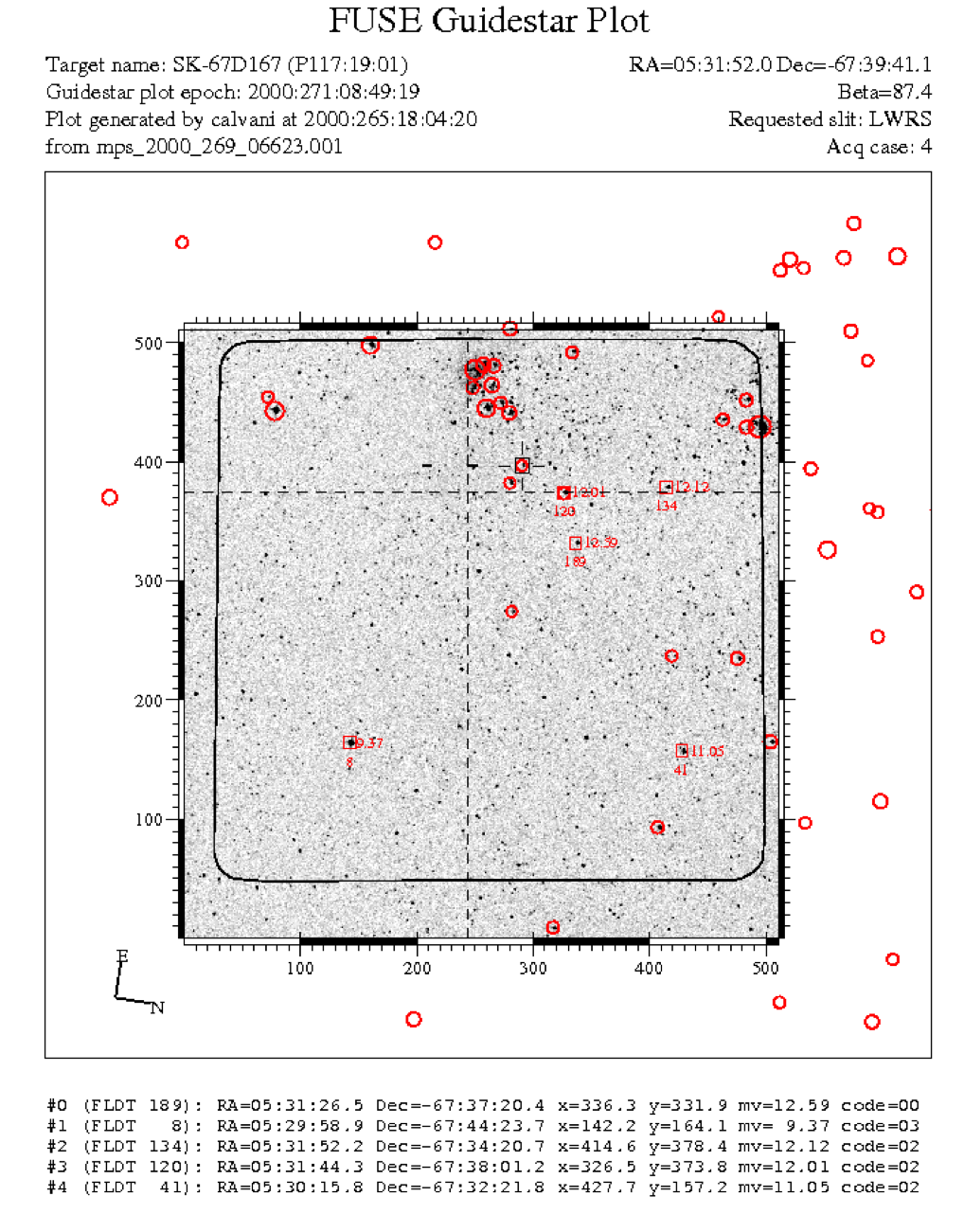
Guide star plots (see Fig. 5.5) were used by the mission planners to identify potential field stars to use for tracking during each observation. Early in the mission, these manually selected stars were actually the ones passed to the ACS and used for tracking, but starting in 2005 the onboard software could find and use autonomously selected stars near each object. Hence, planners simply made a sanity check for available guide stars. The guide star plots show objects from the HST Guide Star Catalog superposed over the expected FES field of view, and show the positions of the apertures. These plots can be useful for interpreting FUSE pointings in crowded fields, especially when used in conjunction with the FES images (remembering that the target may be in the aperture, and thus not visible to the FES). The indicator of North and East on the guide star plots is also useful for interpreting the actual FES images obtained for an observation.
As with other FUSE products, guide star plots evolved in format over the mission, but most of the information given on the plots is straightforward to interpret. The location of the requested aperture is indicated as a box with cross-hairs, and the acq_case codes shown are the same ones used on the MPS plots (see section directly above). The FLDT numbers used to identify certain stars, and listed at the bottom of the plots, refer to an internal numbering system used by the mission planners. Guide star plots for each observation are accessible from the MAST preview pages.
 |
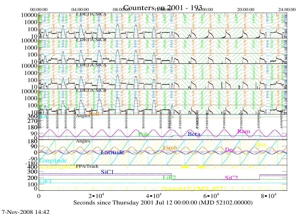
These plots show the actual on-orbit sequence of FUSE activities, all orbital events, and any
anomalies that occurred, with each plot covering a 24-hour period. To the "Intermediate"
and "Advanced" user, these
plots will be useful for placing observations into context since they provide a quick visual assessment
of the actual execution of a given observation and indicate various times associated with each observation
(i.e., high-voltage status, SAA passage, etc...) Figure 5.6 displays an example of
such a plot. (For more details on the content of these
plots and their generation, the user is referred to the
Instrument Handbook (2009)). Each file contains 4 sets of plots
with the count rates for SiC, LiF, FEC, and ACS counters. A brief description of
the SiC plot is provided below. From top to bottom, one can read the following:
Subplots 1-4 show for segments 1A, 1B, 2A, 2B the:
count rate (black); high voltage (red if nominal, blue if not); SAA times (blue horizontal shading);
science data taken (green shading). The OBSID, target, TTAG/HIST flag, and aperture are also
shown if the data are available; low limb angle
times (orange shading); and low ram angle times (purple shading).
Subplot 5 shows the:
Pole angle; Beta angle; Ram angle; Roll; RA; and OBSID (this will be marked at the time when
the observation script began, which is normally well before the actual observation start time).
Subplot 6 shows the:
latitude; longitude; limb angle; Dec; and Day/Night Flag (shaded yellow if Day)
Subplot 7 shows the:
FPA positions; QMEAS flag (scaled); and AT_CMD_ATT flag (scaled).
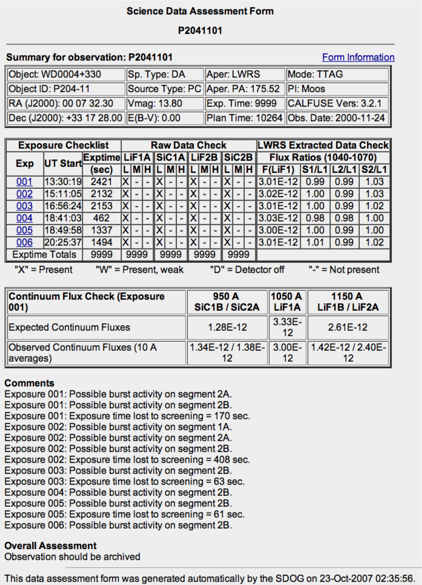
Science data assessment forms, or SDAFs, were used internally by the operations team to provide a quick look assessment of science data quality for each observation. The assessment process was an important part of identifying problems, and if need be, placing revised observations back into the scheduling pool for timely re-execution. The SDAFs are available through the MAST Preview pages for each observation and provide some insight into how a given observation actually executed on-orbit in comparison to how it was planned.
Automated checking routines populated the majority of each SDAF. The software used information from the file headers, some of which was supplied by the user, and compared it to the actual data from each exposure to produce an overview of the success of the observation. This automated process was geared toward the typical FUSE target, which is to say, a moderately bright continuum source. The checks looked for the target in the expected aperture for all four channels and compared the exposure levels to provide an assessment of channel alignment. Hence, very faint sources and emission-line objects could look problematic to the automated process when in reality they might be just fine. Also, the software assumed that LiF1 was the guiding channel, and made comparisons of the other channels to LiF1. After July 12, 2005, when the guiding channel changed to LiF2 (i.e. to FES B), the software was not updated. Hence, some comparisons shown in the SDAF need to be taken in the context of the larger picture of FUSE operations. They are a useful, but imperfect, record of initial data quality assessment.
A brief description of each section of an SDAF is given below. An example SDAF is shown for reference in Fig. 5.7.
Summary Information: A table at the top of each SDAF provides summary information about the target and the observation, populated automatically from the file headers. Included are the actual achieved time for the observation as compared with the planned time in the timeline. If problems occurred, or if the processing deleted some data sections as bad, these numbers will be different.
Exposure checklist: This tabular section contains one line for each exposure in the observation. At left are the UT start time of each exposure and the integration achieved in that exposure (from the LiF1A segment). In the middle are the ŇRaw Data CheckÓ blocks that use various symbols to indicate the presence (or absence) of data in the various channels and apertures. This raw data check scans all apertures for TTAG data or the primary aperture for HIST data. The key for this section includes:
The example in Fig. 5.7 shows the source present in all exposures
and in all LWRS (prime) apertures. Also, since the exposure times are the same for all
four apertures, there was apparently no drifting of the target in and out of the various
apertures. This is also confirmed by the Extracted Data Check blocks to the right,
which show a consistent signal in LiF1 in all channels, and ratios near unity compared to the LiF1
for the other channels throughout the exposures. In crowded fields and for TTAG
exposures, sources could sometimes be present in the non-prime apertures. If this was
true, one would also see "X" or "W" in other apertures where flux was present. Finally,
if telemetry indicated that the high voltage was down for a particular channel, the
indicator would show "D" and no data would be present in that channel for that exposure.
Continuum Flux Check: Part of the exposure checklist also includes a check on the CalFUSE
pipeline extracted output. This section of the SDAF provides a sanity check
against expectations. For each FUSE target, the observer was asked to provide
continuum fluxes at 950, 1050, and 1150 Å (if appropriate for their target type). The
Continuum Flux Check box just makes a simple comparison of actuals against these
expectations, and performs some comparisons between channels. The LiF1 fluxes are used as
a benchmark. If the flux in another overlapping segment is significantly lower or higher,
then a comment is added later in the form (see below). Also, if flux is detected in the
extracted spectrum at a level greater than the LiF1 level and the raw data indicates that
no data should be present, a warning is issued in the comments. In some cases, observers
had only rough estimates of the expected fluxes, so it is not uncommon to see significant
differences from unity. Also, lower values could indicate channel drifts are affecting
the observation, especially for MDRS and HIRS observations. (Note again that data taken after 12
July 2005 did not use the LiF1 channel for guiding, but the SDAF software was never
updated for this.)
Comments Section: This section contains a number of comments, exposure by exposure,
generated by the CalFUSE processing sotfware as it processed the data. The example shows
comments related to the presence of bursts and time removed because of them. Sometimes
a general alert will be present in red, indicating a flux much lower than expected or
similar criterion that can be measured automatically. Usually such problems would already
be obvious from inspection of information at the top of the SDAF, but the red comment
flags the probable causes of problems specifically. Warnings are more serious than
alerts, and when initially issued, would prevent archiving of the data until an
assessment was made by FUSE personnel. (Few if any warnings remain in the
final SDAF forms generated in the reprocessing performed at the end of the mission, however.)
For observations made in the MDRS or HIRS apertures, the standard procedure involved performing a peak-up acquisition (sometimes multiple times per orbit) to align the channels at the beginning of the observation. When this is the case, one will find an ascii peak-up table appended to the end of the SDAF for that observation. This information is provided for completeness, but it is not expected that most users will need it for analyzing their data.