GOAL: To determine how well the WFC3 "Sloan" filters (F475W, F625W, and F775W) mimic the real Sloan filters (g, r, and i).
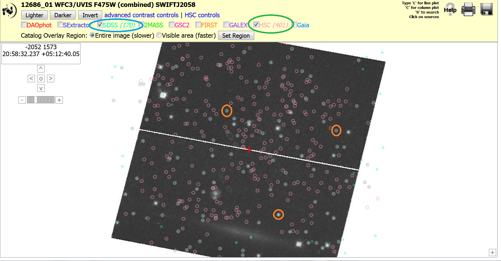
Using the HLA, check whether there is data in both the HSC and SDSS for the F475W filter in the field of GRB110328A (SWIFT J2058+05). To see this, display the image hst_12686_01_wfc3_uvis_f475w (RA=20:58:20.07, Dec. = 05:13:22.0) using the HLA interactive viewer. Click on the SDSS catalog (blue) and the HSC (green) and note that there are stars that are in both catalogs (orange).
For the F625W and F775W filters, the field of 3C58 (RA=02:05:42.05, Dec. = +64:48:38.8) has the necessary data.
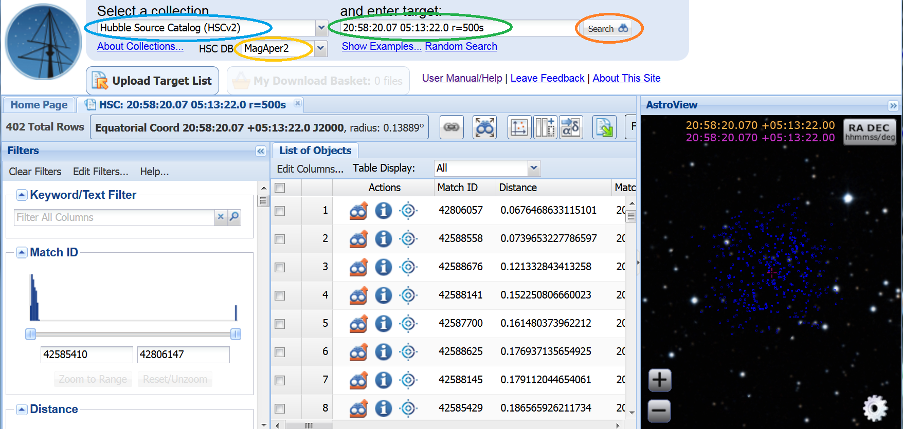
Use the pull down menu under Select Collection to choose the HSC
(blue).
Enter the coordinates (from above) and search radius of 500s in the Search
box (green); note that you will need to
do this for each field. Perform the
search by just hitting a carriage return or by clicking on the
 icon (orange).
The results are displayed in the List of Objects, while the AstroView
window shows the objects against the DSS image.
icon (orange).
The results are displayed in the List of Objects, while the AstroView
window shows the objects against the DSS image.
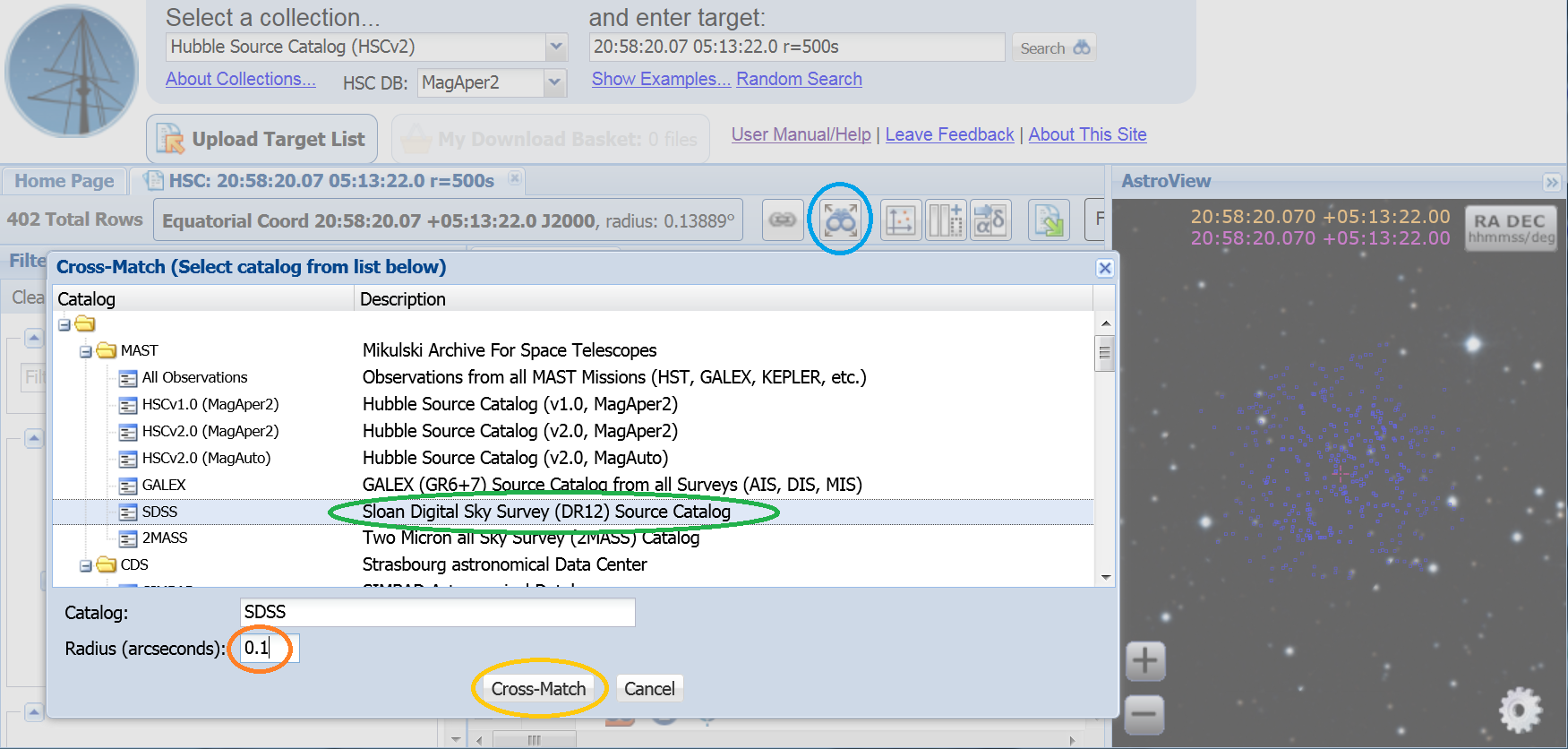
To cross-match the HSC catalog with another catalog, click on the
 icon (blue) and select the SDSS catalog
(green). Set the matching radius
to 0.1" (orange) and hit Cross-Match
(yellow). This will create a new tab
with the cross-matching results.
icon (blue) and select the SDSS catalog
(green). Set the matching radius
to 0.1" (orange) and hit Cross-Match
(yellow). This will create a new tab
with the cross-matching results.
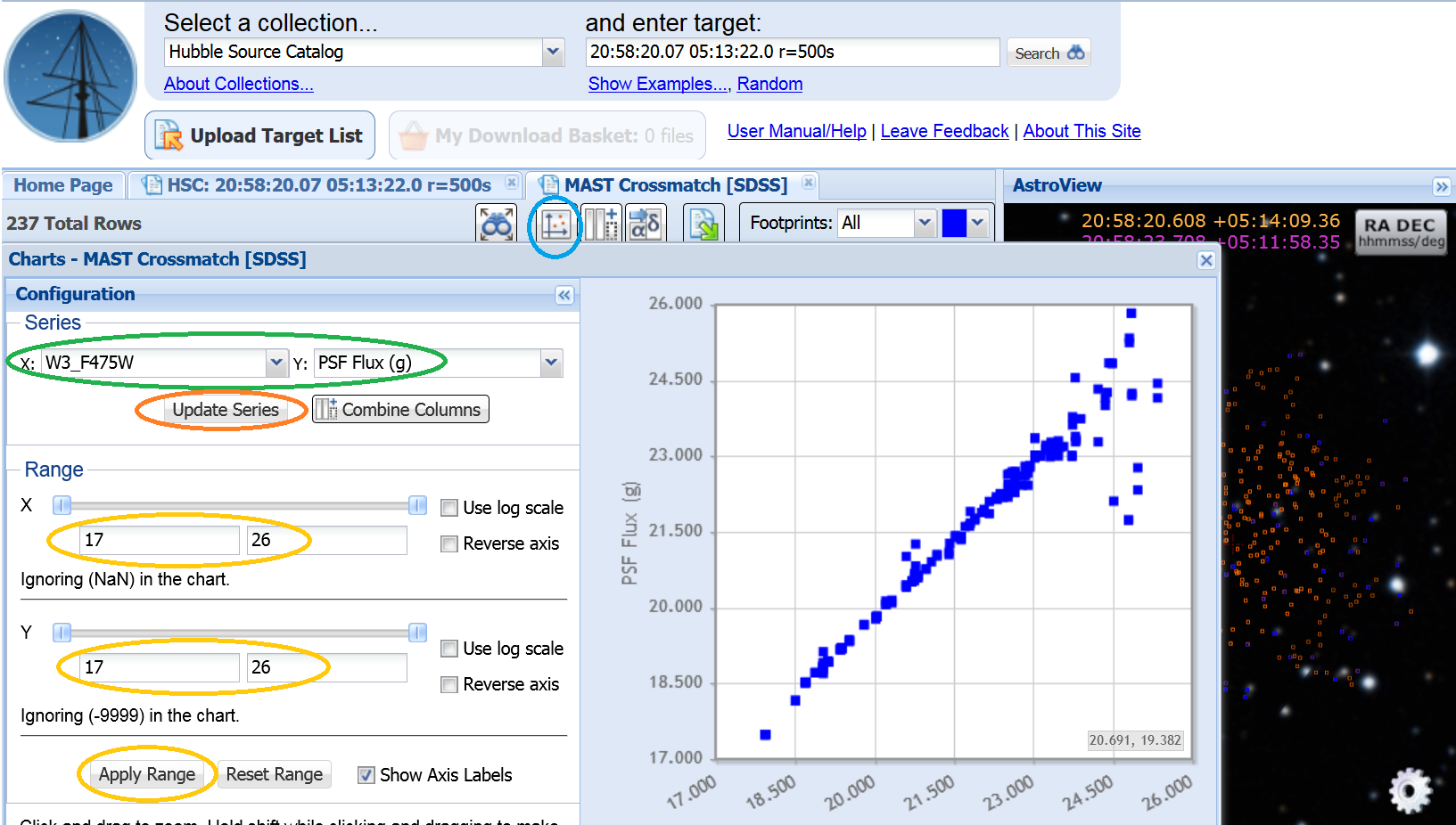
Scroll out to see all the columns. Note that for the first item (Match ID = 22146135), WFC3_F475W = 22.02 and PSF Flux(g) = 21.88.
Make a plot of the WFC3 magnitude against the SDSS magnitude by clicking on
the  icon (blue). Under Configuration, select
X=W3_F475W and Y=PSF Flux(g) (green), then
click on the Update Series button
(orange); you MUST also set the X and Y
range, and then click Apply Range to cover the same values (yellow).
icon (blue). Under Configuration, select
X=W3_F475W and Y=PSF Flux(g) (green), then
click on the Update Series button
(orange); you MUST also set the X and Y
range, and then click Apply Range to cover the same values (yellow).
The fits look pretty good (there is good agreement between the WFC3 Sloan F475W and the SDSS g filters), although the fit is significantly worse at the faint end. If we go to the Filters column (on the far left) and restrict the Concentration Index (CI) values to be less than 1.3 (blue) to eliminate potentially blended objects, then the fit improves significantly.
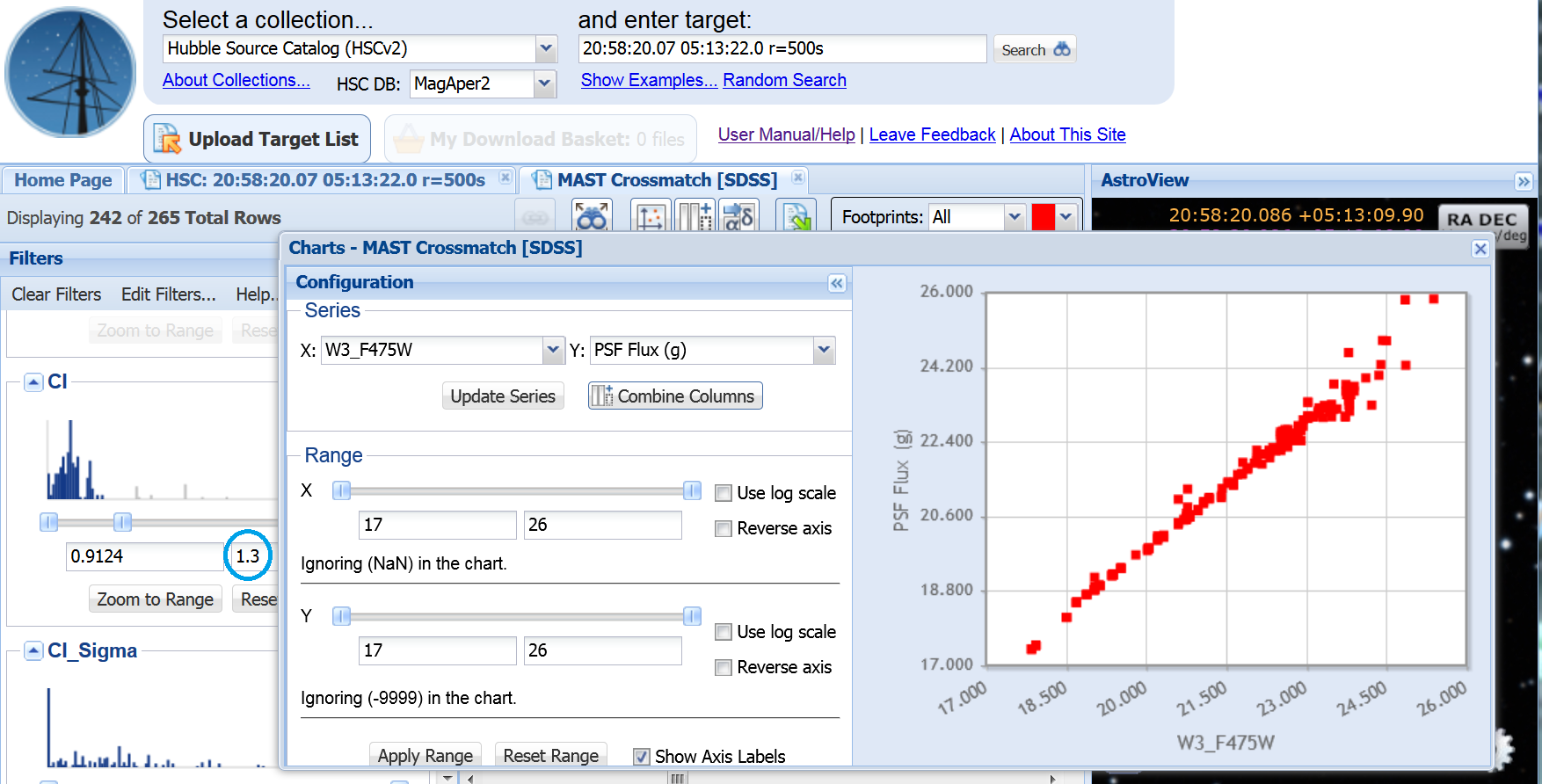
Note that there is a systematic difference of a one to two-tenths, with the SDSS magnitudes being brighter. This is due to a number of different effects that include:
See Whitmore et al. 2015 for a further discussion of comparisons with SDSS and a similar comparison using galaxies in the Hubble Deep Field.
You can download the matched table using the
 icon to do
further analysis using your favorite analysis system.
icon to do
further analysis using your favorite analysis system.
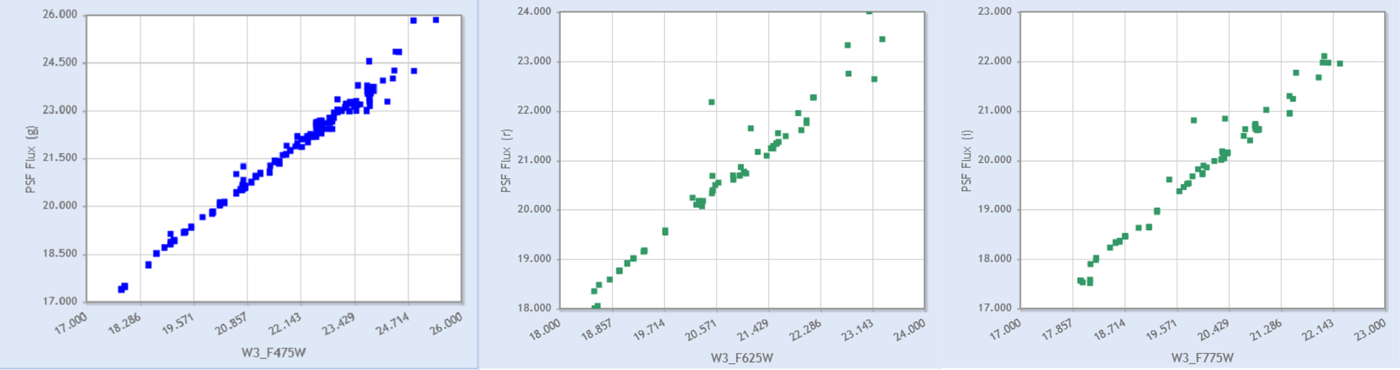
Perform the same steps for the W3_F625W/Sloan r and the W3_F775W/Sloan i pairs (using the 3C58 dataset mentioned above) .
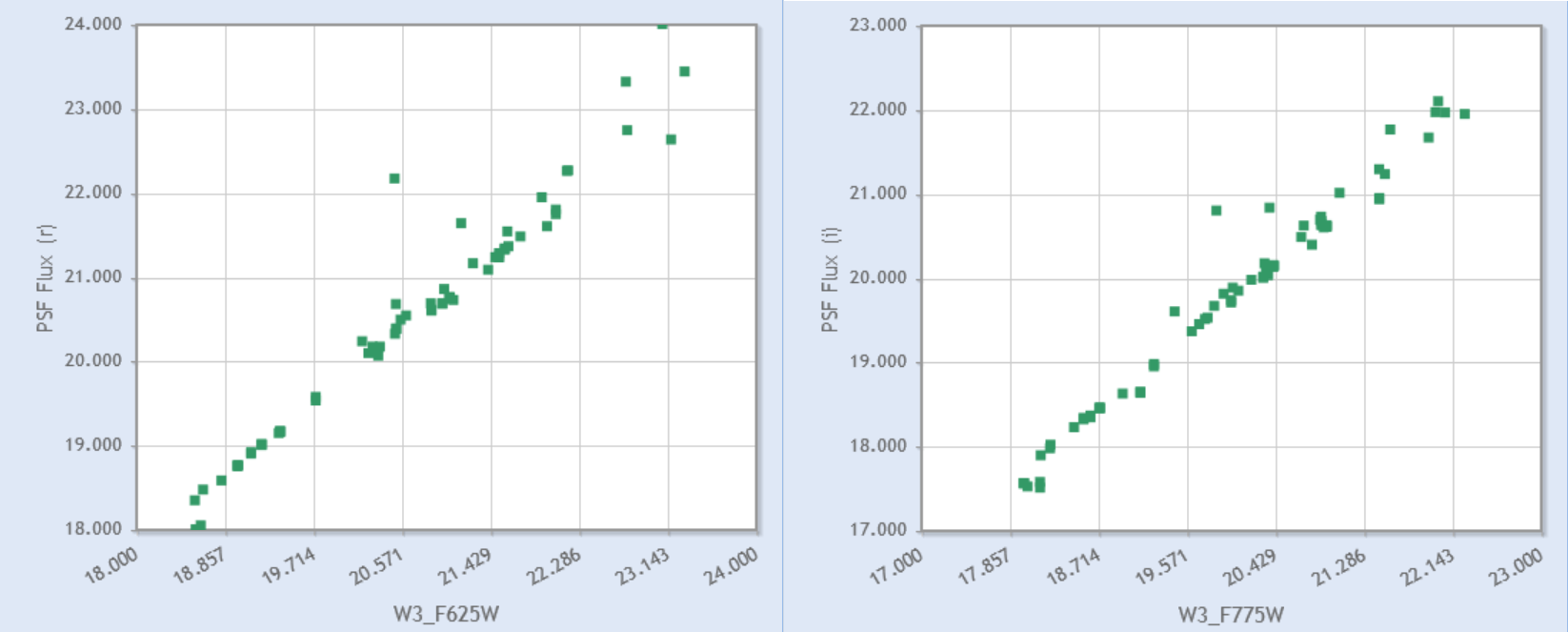
As with the F475W/Sloan g filters, the WFC3 and SDSS magnitudes are in good agreement.