This is a description of an older version of
the Hubble Source Catalog.
The
current version is preferred for most purposes.
A Hubble Source Catalog (HSC) Use Case
Example #3: Using the Discovery Portal to search for Variable Objects in the HSC
(Time Variability in the dwarf irregular galaxy IC 1613)

|
GOAL: This tutorial shows you how to use the
MAST Discovery Portal to search for variable objects in the HSC.
SCIENCE CASE: The science case is searching
for variable objects (i.e. in the irregular galaxy IC 1613; Bernard et al. 2010, ApJ 712, 1259).
Step 1 - Go to the
MAST Discovery Portal.
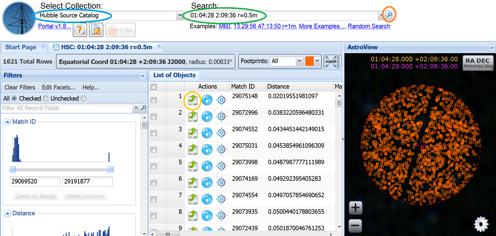
Use the pull down menu under Select Collection to choose the HSC
(blue).
Enter (you can just cut and paste if you like) the coordinates and
search radius (i.e. 01:04:28 2:09:36 r=0.5m)
in the Search box (green); note that
this is in the outskirts of IC 1613.
Perform the search by just hitting a carriage return or by
clicking on the  (orange).
The results are displayed in the List of Objects, while the AstroView
window shows the objects against the DSS image. The left column is a
series of Filters that can be used to refine the data selected.
|
 |
The DSS is not helpful (the outskirts of the galaxy are very faint), so
we need to load an HST image. Click on the Load Detailed Results
 icon (yellow in the previous figure) to
bring up the HSC Detailed Form.
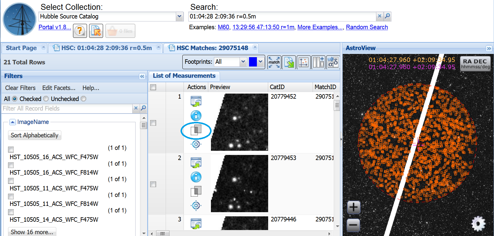
Click on the Toggle Overlay Image
 icon
(blue) to load the HST
image. Note that you can click on the Preview image to bring up the
HLA interactive viewer to get a better look at the HST data.
 |
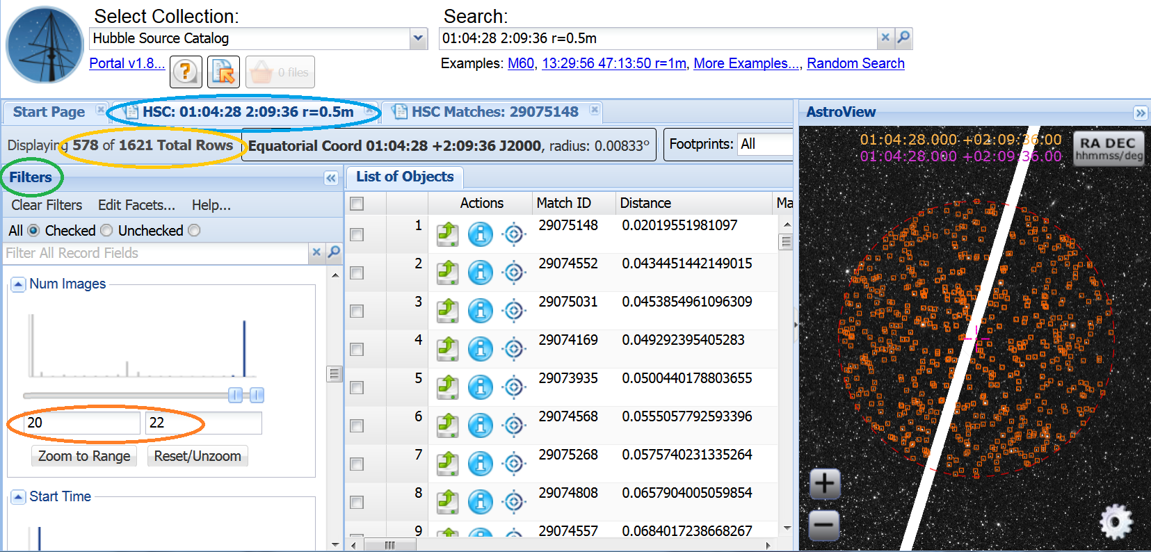
Step 2 - Go back to the search tab ( blue),
scroll down the Filters section ( green)
on the left to the Images block, and
move the sliders to select sources with 20 to 22
images ( orange). Note that fewer rows
are now displayed ( yellow), and that the
image also shows fewer targets.
|
 |
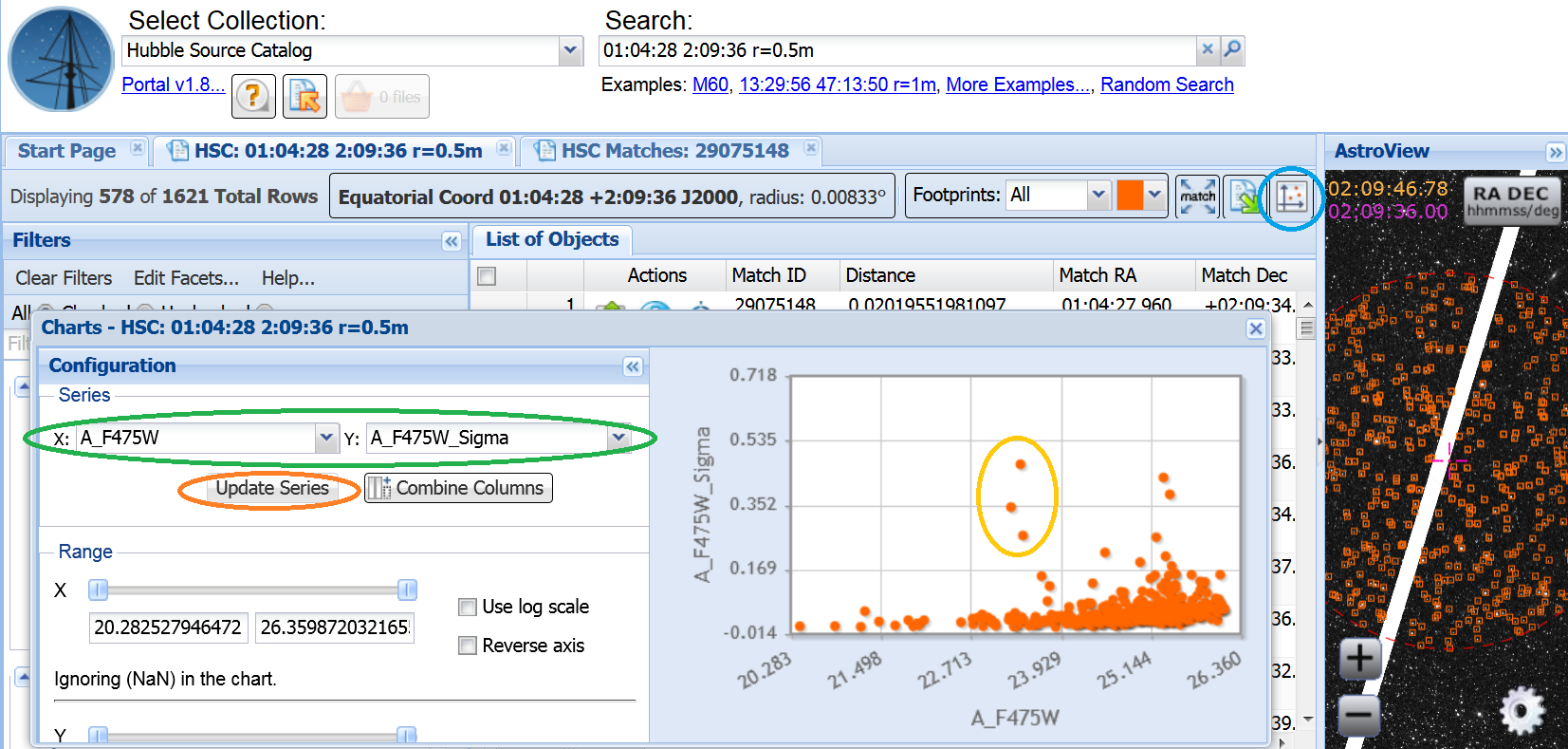
Step 3 - Make a plot by clicking the
 icon
( blue). Under Configuration, select
X = A_F475W and Y = A_F475W_Sigma ( green).
Click on the Update Series button ( orange)
to plot the ACS F475W magnitudes vs. the RMS scatter for each data point.
The potential variable stars have large Sigmas ( yellow).
|
 |
Step 4 - Select a specific source by clicking on it (i.e. 23.4, 0.47)
( blue). This will highlight the object in
the AstroView window
( green), and bring the source to the
top of the List of Objects
(i.e. matchID=29073890) ( orange).
|
 |
Step 5 - You can examine the 21 measurements and images that went
into the MatchID=29073890 by clicking on the first
 icon under
Actions ( yellow in the previous figure)
in the List of Objects. This brings up the HSC Detailed Form data. Note that
there is a crosshair on the target ( green).
|
 |
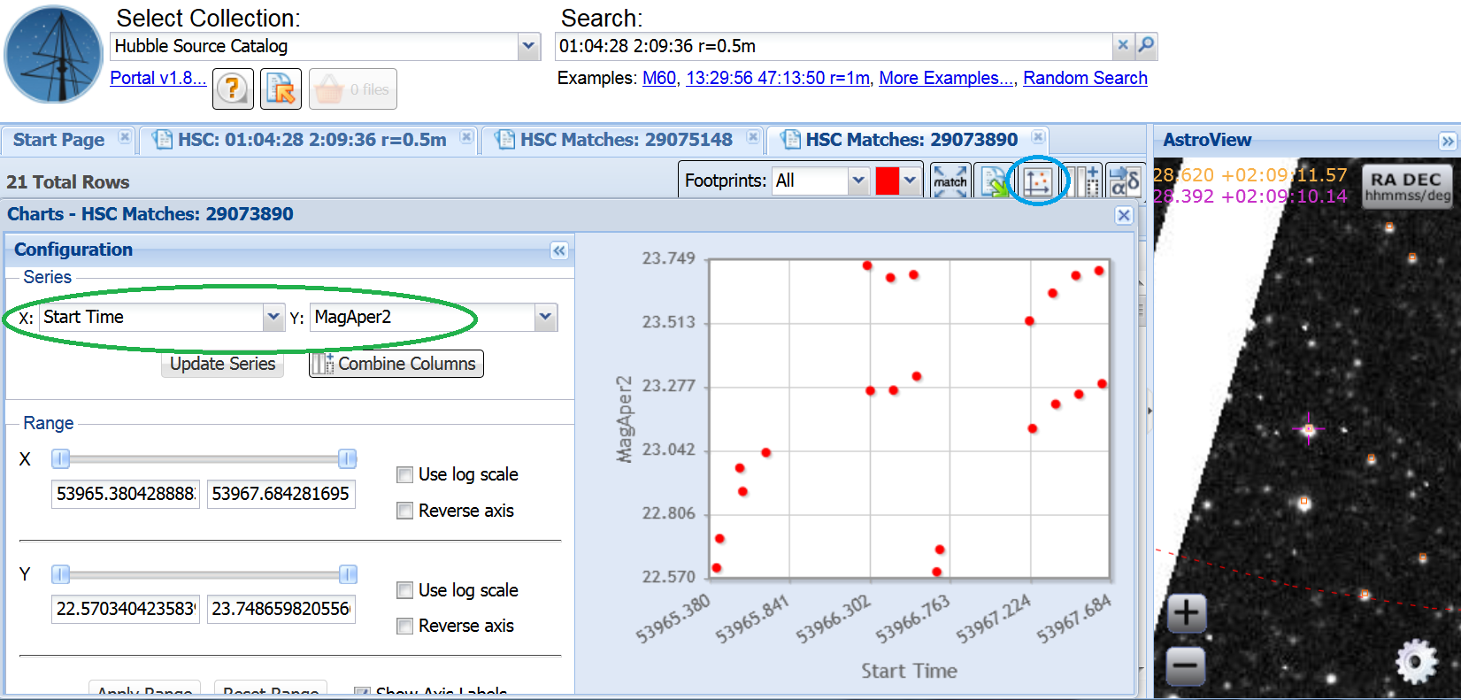
The light curve can then be plotted using the
 icon
(blue) again with
X = Start Time and Y = MagAper2 (green).
 |
Step 6 - While there is clear variability, the plot is confusing
since there is both F475W and F814W data plotted.
To look at only one magnitude at a time, go to the Filters section on
the left and scroll to the Filter area and select one of the
filters ( blue).
Note that the plots (below) have fewer points,
and that this object is clearly variable in the both filters.
The fact that the shape of the
light curves are similar (although the amplitude is different)
indicates that the variability is real.
|
 |
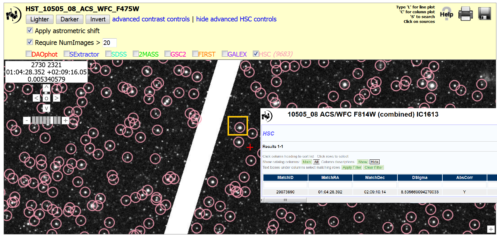
Step 7 - To make sure the variability is real (i.e. that there are
no image artifacts "causing" the magnitude scatter), you should examine
the images. Clicking on
the image in the Preview column in the List of Measurements will bring up the HLA's Interactive display. Show
the advanced HSC controls ( blue) and
select Apply astrometic shift,
as well as set Require NumImages to be greater than 20 ( green).
Click in the HSC box ( orange) and the HSC
catalog is overlaid on the image. Find the star of interest (click on the
object to verify the identification ( yellow))
and verify that the object is free from
artifacts. Ideally, you would do this for all the images.
|
 |
You could also make an F475W - F814W (B-I) column (by using the
Combine Columns option ( blue)) and
plot the color-magnitude diagram; see Use Case #5 for more on
making a CMD. Note that the 3 variable candidates
( green) fall in the instability
strip, further suggesting that they really are variables.
|
 |


 (orange).
The results are displayed in the List of Objects, while the AstroView
window shows the objects against the DSS image. The left column is a
series of Filters that can be used to refine the data selected.

 icon (yellow in the previous figure) to
bring up the HSC Detailed Form.
Click on the Toggle Overlay Image
 icon
(blue) to load the HST
image. Note that you can click on the Preview image to bring up the
HLA interactive viewer to get a better look at the HST data.


 icon
(blue). Under Configuration, select
X = A_F475W and Y = A_F475W_Sigma (green).
Click on the Update Series button (orange)
to plot the ACS F475W magnitudes vs. the RMS scatter for each data point.
The potential variable stars have large Sigmas (yellow).


 icon under
Actions (yellow in the previous figure)
in the List of Objects. This brings up the HSC Detailed Form data. Note that
there is a crosshair on the target (green).

 icon
(blue) again with
X = Start Time and Y = MagAper2 (green).
