FAQ - General
-
What is the Hubble Source Catalog (HSC)? What data does it contain?
The Hubble Source Catalog (HSC ) combines the tens of thousands of visit-based, general-purpose source lists in the Hubble Legacy Archive (HLA) into a single master catalog.
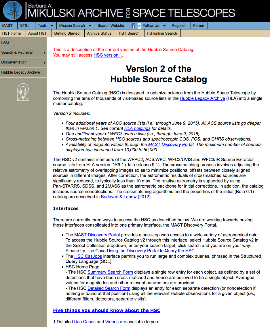
Version 1 of the HSC contained members of the WFPC2, ACS/WFC, WFC3/UVIS, and WFC3/IR Source Extractor source lists from HLA version DR8 that were public as of June 1, 2014.
Version 2 contains source lists from the same instruments, but using HLA version DR9.1 images (i.e., public as of June 9, 2015.)See What is new in version 2 for more details about improvements and enhancements made to Version 2. Both Version 1 and Version 2 of the HSC will continue to be available.
-
What is new in Version 2 of the Hubble Source Catalog?
The primary new items for Version 2 are:
-
1. The addition of approximately four more years worth of ACS source lists (i.e., using data public as of June 2015). In addition, all ACS source lists are approximately one magnitude deeper than in version 1.
-
2. The addition of approximately one more year of WFC3 source lists (i.e., using data public as of June 2015).
-
3. Spectroscopic cross-matching between COS, FOS, and GHRS data and HSC sources is now available.
-
4. A "normalized" value of the Concentration Index, still denoted as CI, in the Summary Form.
-
5. Availability of magauto values through the MAST
Discovery Portal.
The maximum number of sources displayed by the Discovery Portal has increased from 10,000 to 50,000.
In January, 2017 a few relatively minor additions were made to the HSC which should not affect most users. These are referred to as Version 2.1 .
-
1. Tables have been made available via HSC CASJOBS providing MEDIAN
rather than MEAN values for magnitudes from the summary form (scroll down to the Instrument_Filter explanation). This can help filter out photometric outleyers.
-
2. A table has been made available via HSC CASJOBS providing
cross-matching between Version 1 and Version 2 sources (i.e., xMatchV1).
-
3. Spectroscopic matches for COS, FOS, and GHRS observations have
been added for Version 2 sources that do not have Version 1 counterparts.
-
What are five things you should know about the HSC?
NOTE: The graphics in this section are from version 1.
1. Detailed HSC use cases and videos are available to guide you.
2. Coverage can be very non-uniform (unlike surveys like SDSS), since pointed observations from a wide range of HST instruments, filters, and exposure times have been combined. However, with proper selection of various parameters (e.g., NumImages included in a match), this non-uniformity can be minimized in most cases. In the example below, the first image (with NumImages > 10) shows a very nonuniform catalog, while the second image (with NumImages > 3) is much better.
3. WFPC2 source lists are of poorer quality than ACS and WFC3 source lists. As we have gained experience, the HLA source lists have improved. For example, many of the earlier limitations (e.g., depth, difficulty finding sources in regions of high background, edge effects, ...) were fixed in the WFC3 source lists for version 1. These improved algorithms have now been included for the ACS/WFC in version 2, but have not been used for WFPC2.
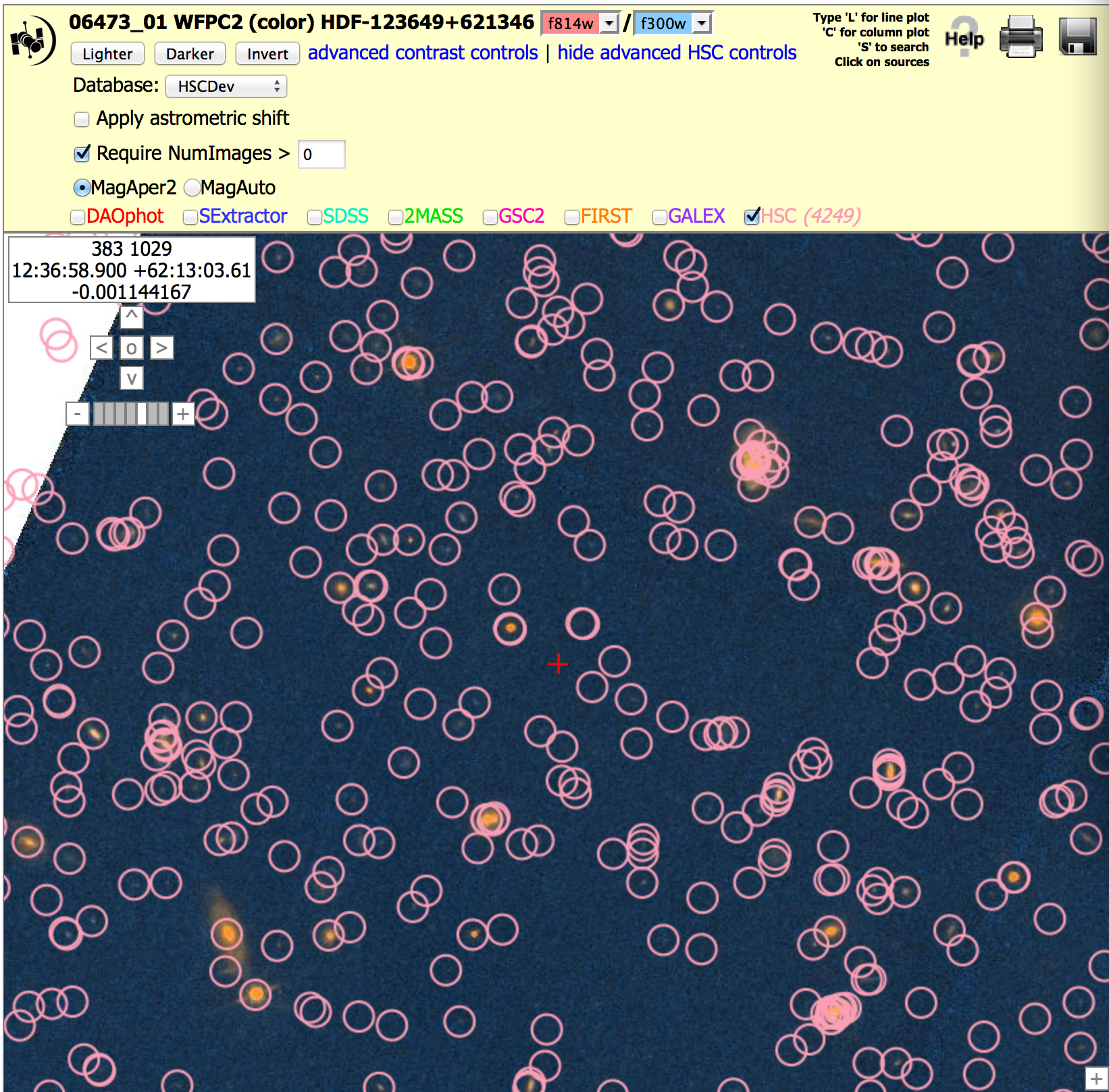
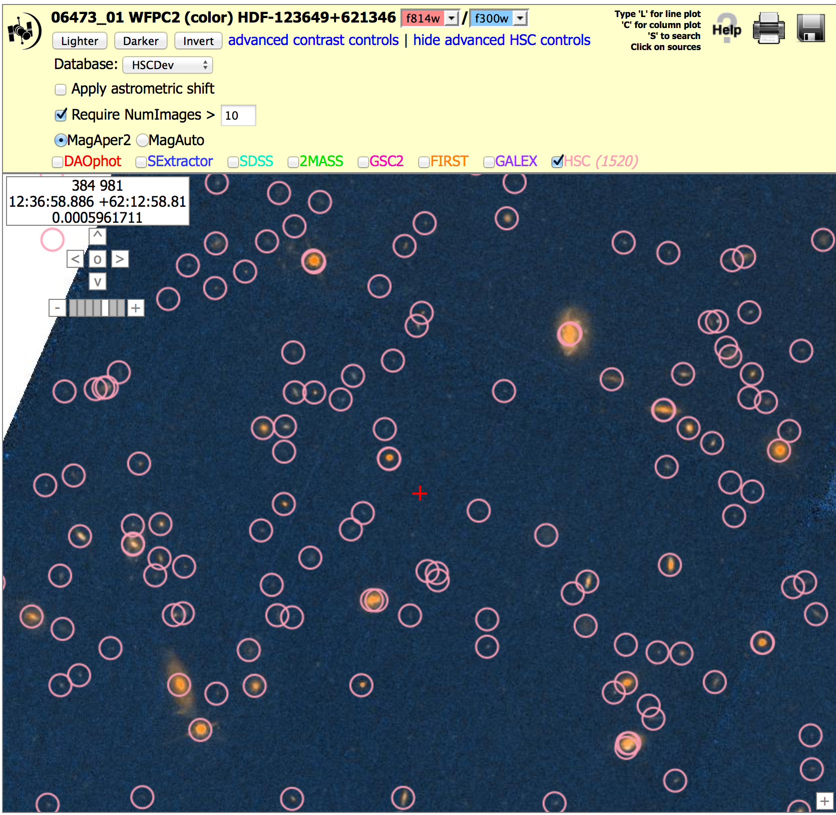
4. The default is to show all HSC objects in the catalog. This may include a number of artifacts. You can request Numimages > 1 (or more) to filter out many of the artifacts. In the example below we show part of the Hubble Deep Field (HDF). With NumImages > 0 on the left, a number of the points look questionable (e.g., several of the circles to the right of the red cross have NumImages = 1 or 2, and look blank). Even the faint sources in this particular field have NumImages in the range 10 - 20, hence a value of NumImages > 10 is more appropriate.
5. The default is to use MagAper2 (aperture magnitudes), generated using the Source Extractor (Bertin & Arnouts 1996) software.
If required for your science needs, you will need to add aperture corrections to estimate total magnitudes. These can be found in the Peak of Concentration Index for Stars and Aperture Correction Table. You can also request MagAuto values if you would like to use the Source Extractor algorithm for estimating the total magnitude. This is especially appropriate for many extended sources.
All HLA (and hence HSC) magnitudes are in the ABMAG system. Here is a discussion of the ABMAG, VEGAMAG and STMAG systems. A handy, though not exact conversion for ACS is provided in Sirianni et al. (2005). The Synphot package provides a more generic conversion mechanism for all HST instruments.
-
Where can I find examples of good and bad regions of the HSC?
NOTE: Unless otherwise noted (in red), the images in this section are from HSC version 1.Good examples:
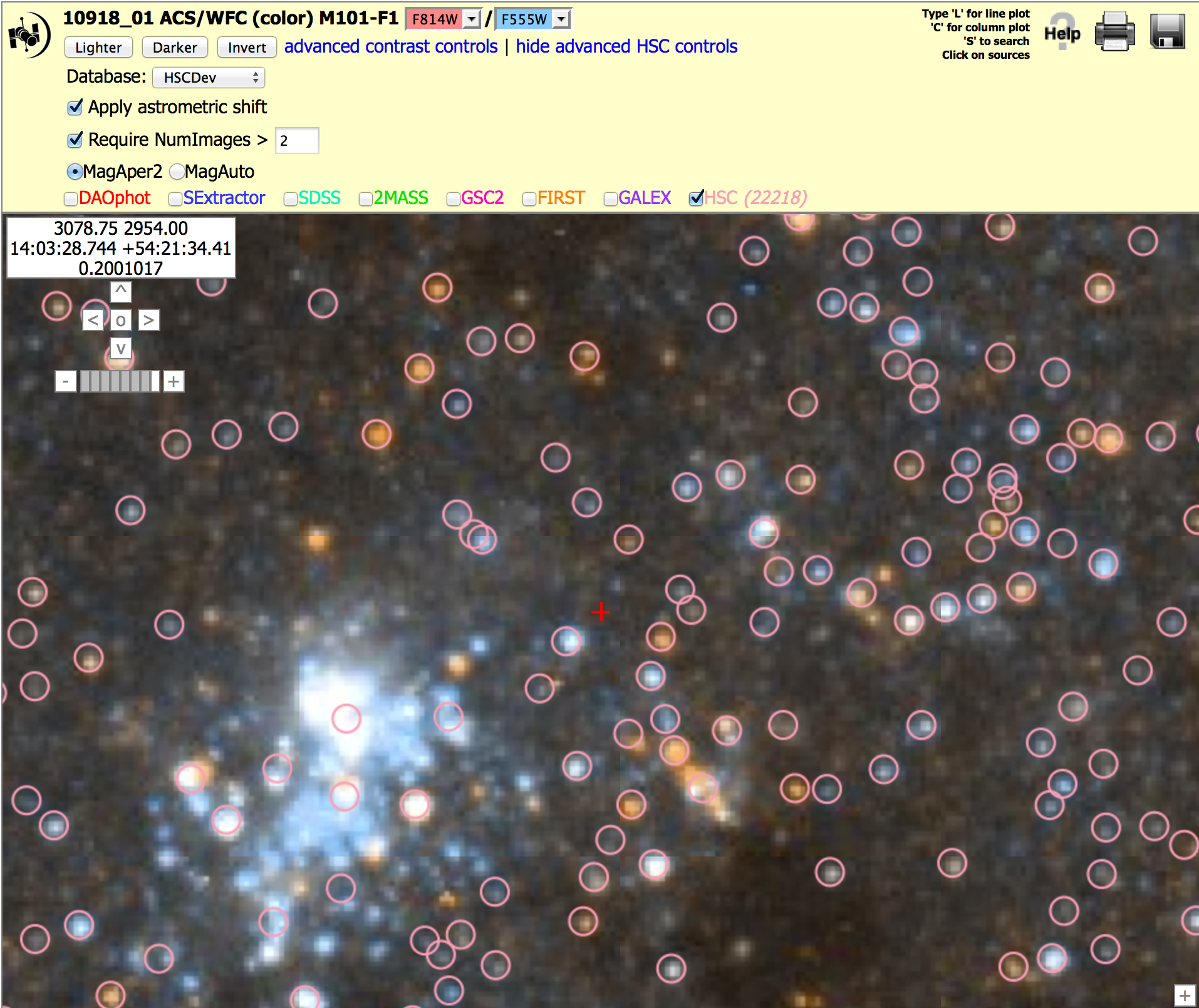
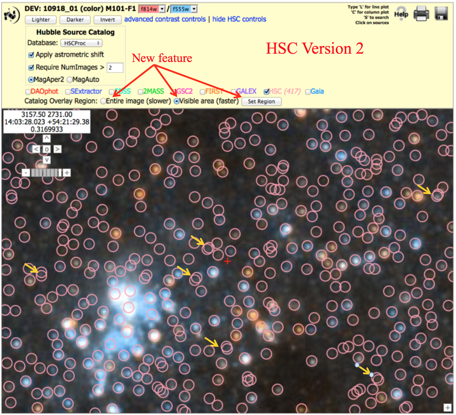
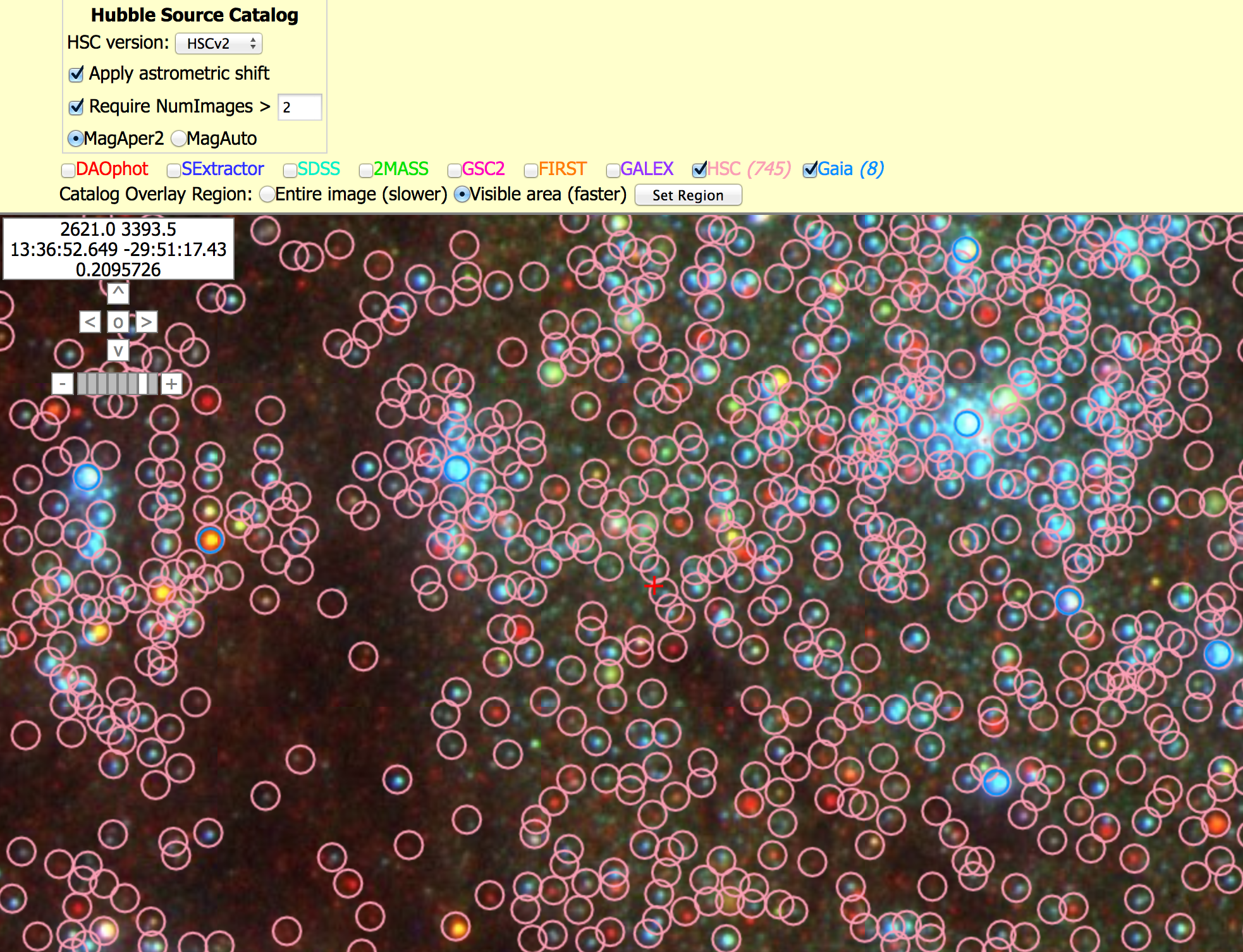
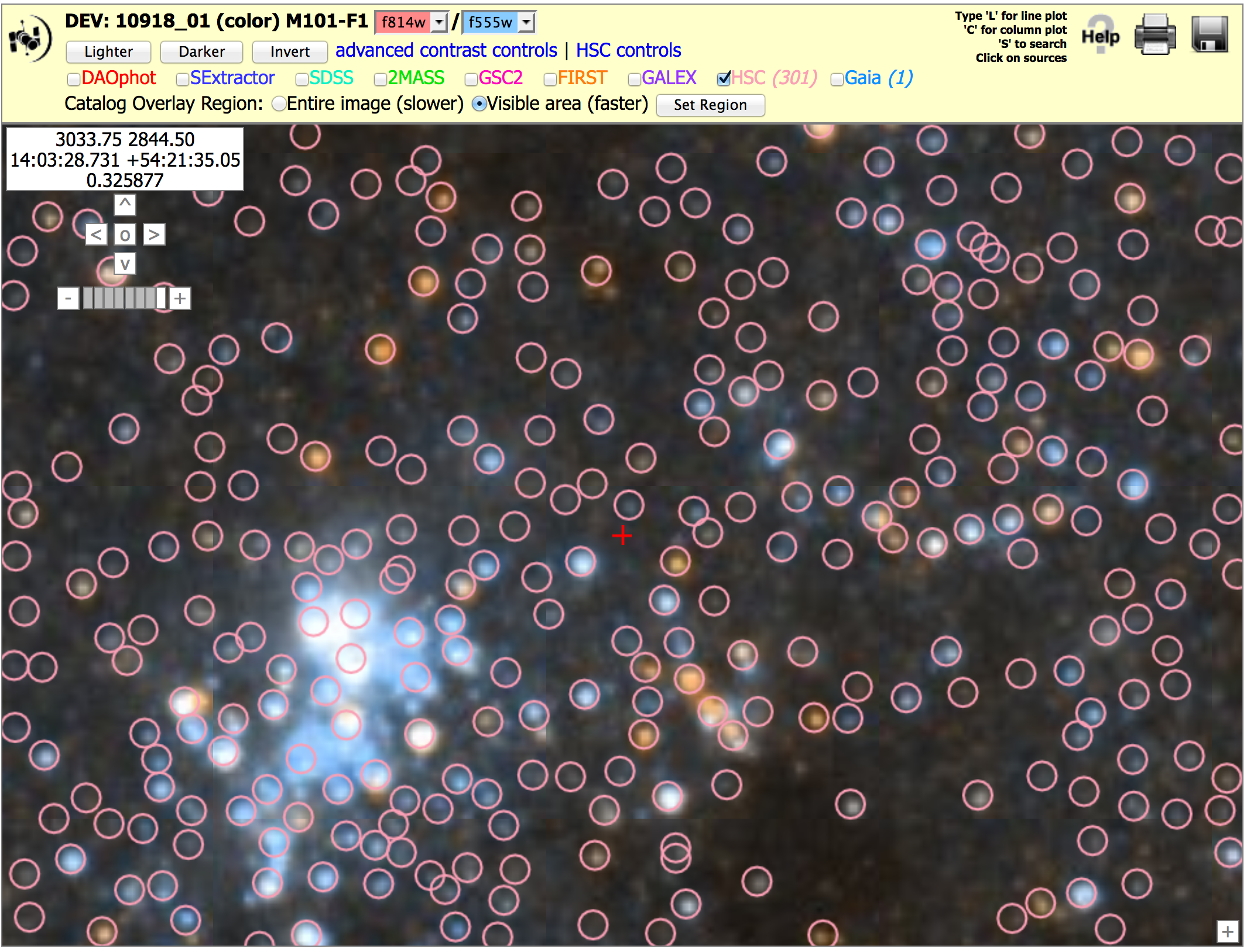
Nearby galaxy: ACS, M101 (10918_01), N > 2 version To get the image below, click on "Advanced HSC controls", then check the box for "Require NumImages > 2", then click on HSC.
Note the yellow arrows that show that there is sometimes more "doubling" seen in version 2 images, primarily because of the inclusion of fainter ACS sources. See known problems #2 for a discussion on doubling.
Note that HSC version 2 has many more sources.
There is also a new feature which allows you to plot only the objects visible in the particular region you have selected. This greatly increases the speed needed to plot the points. Click on either the "Entire image" or "Visible area", and then click "Set Region".
Note that it is now possible to overlay Gaia sources.
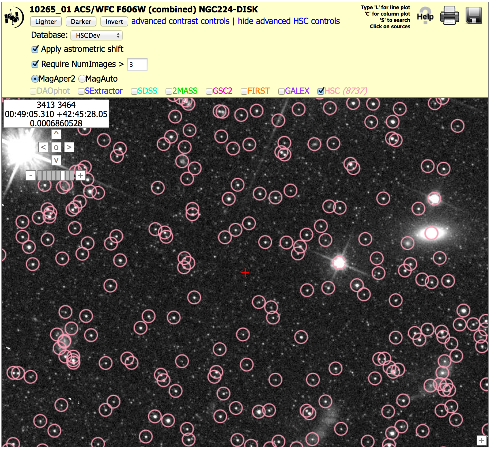
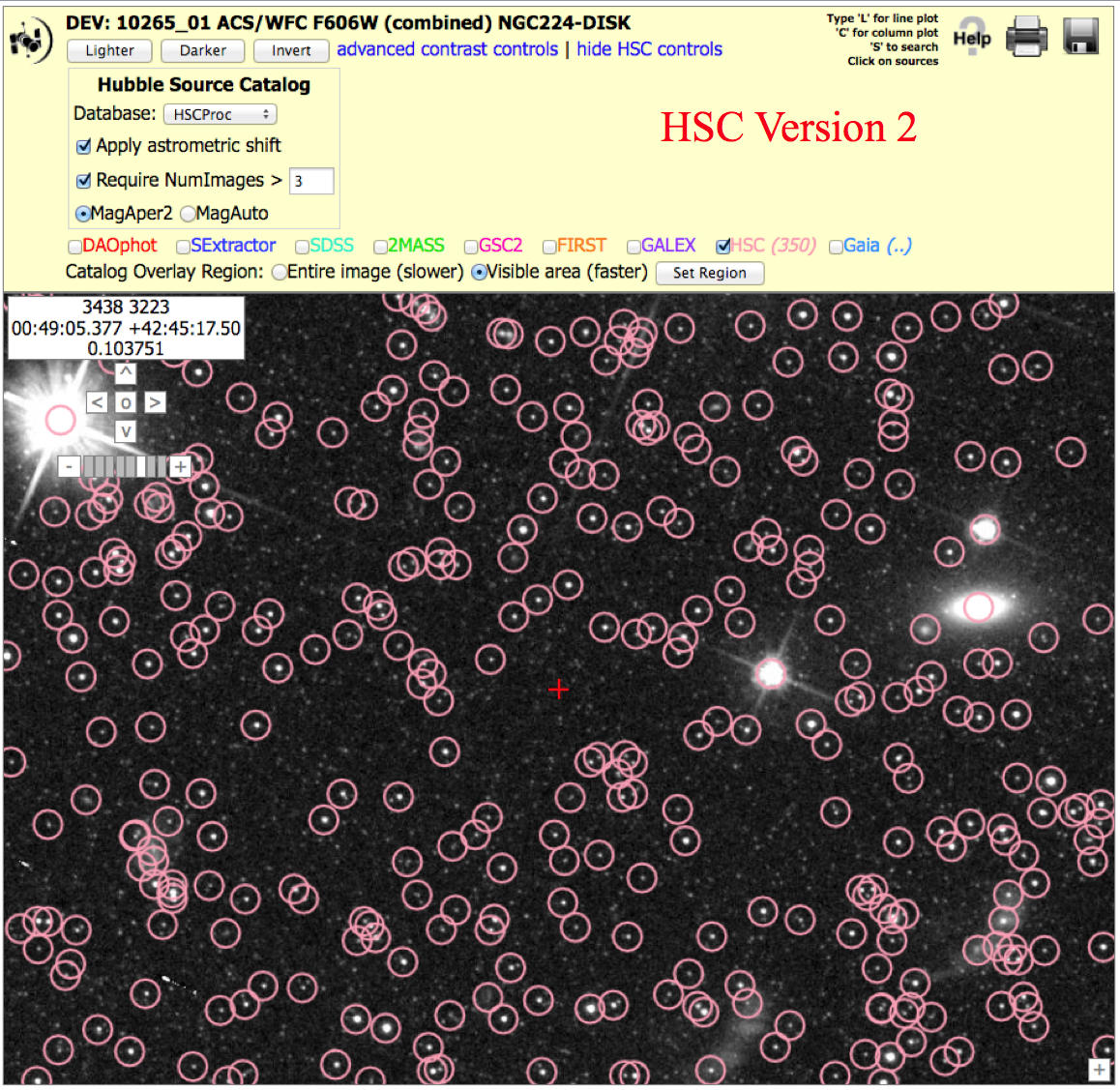
Star field: ACS, M31 (10265_01), N > 3 version To get the image below, click on "Advanced HSC controls", then check the box for "Require NumImages > 3", then click on HSC.
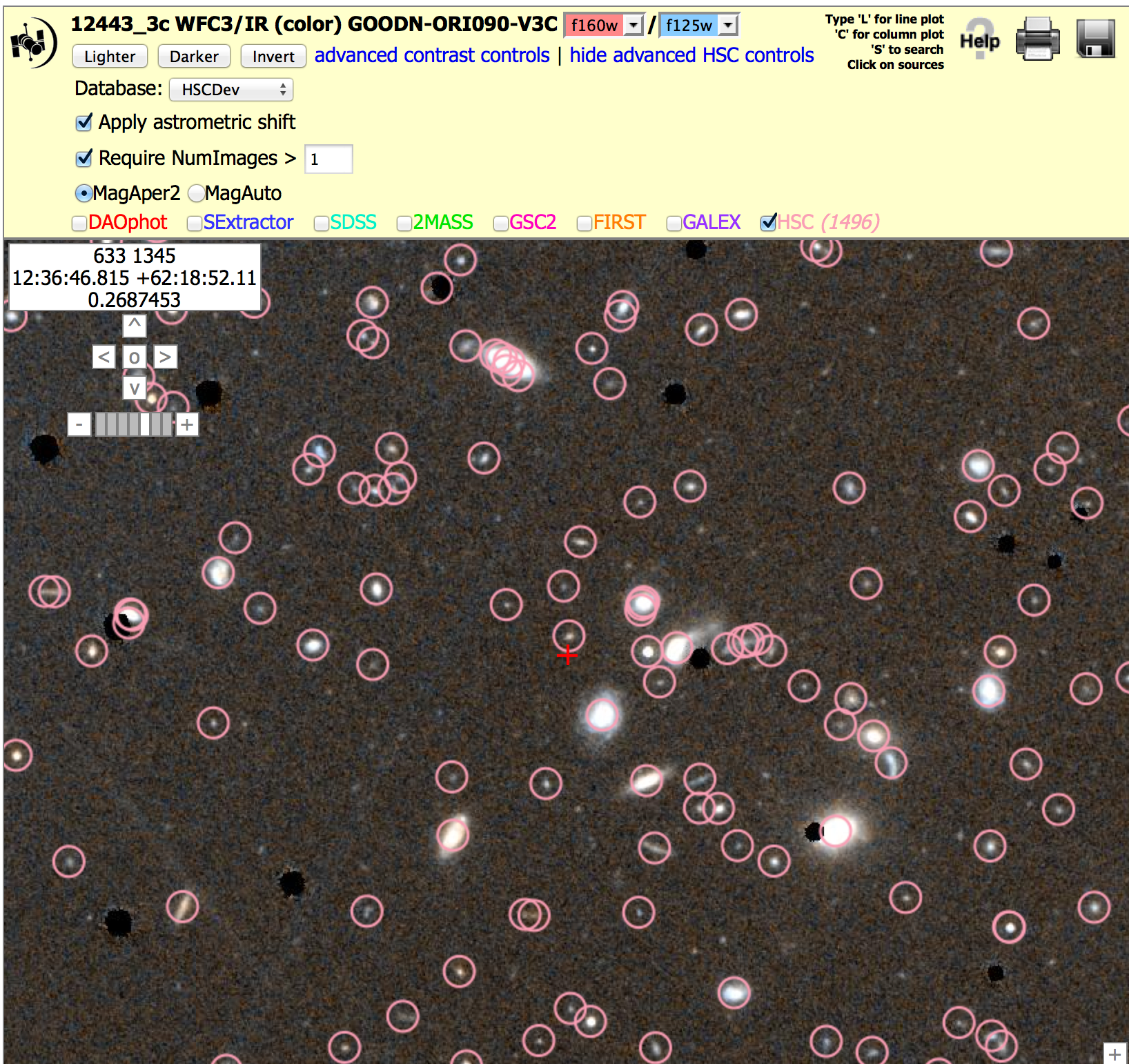
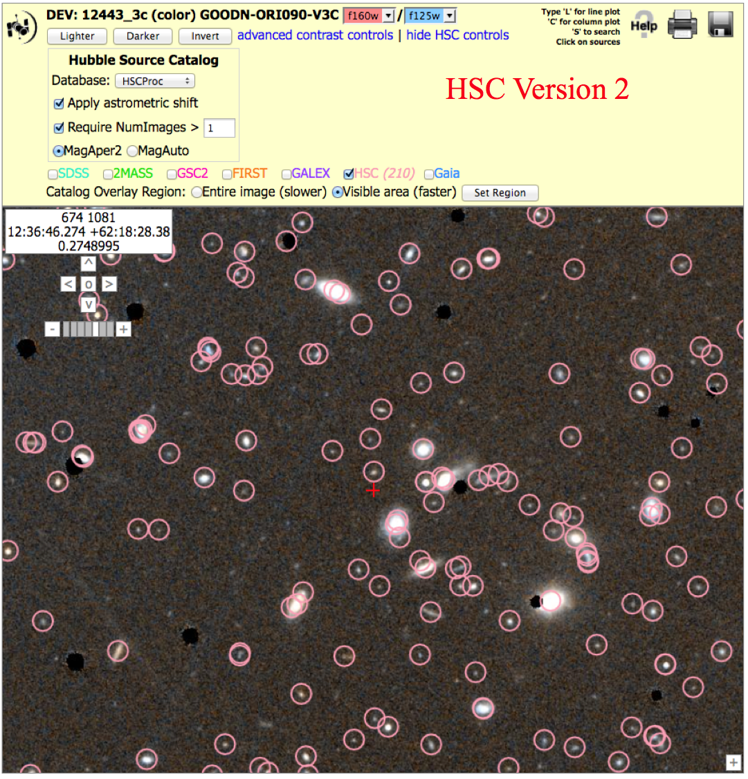
Field of faint galaxies: WFC3/IR, (12443_3c), N > 1 version To get the image below, click on "Advanced HSC controls", then check the box for "Require NumImages > 1", then click on HSC.
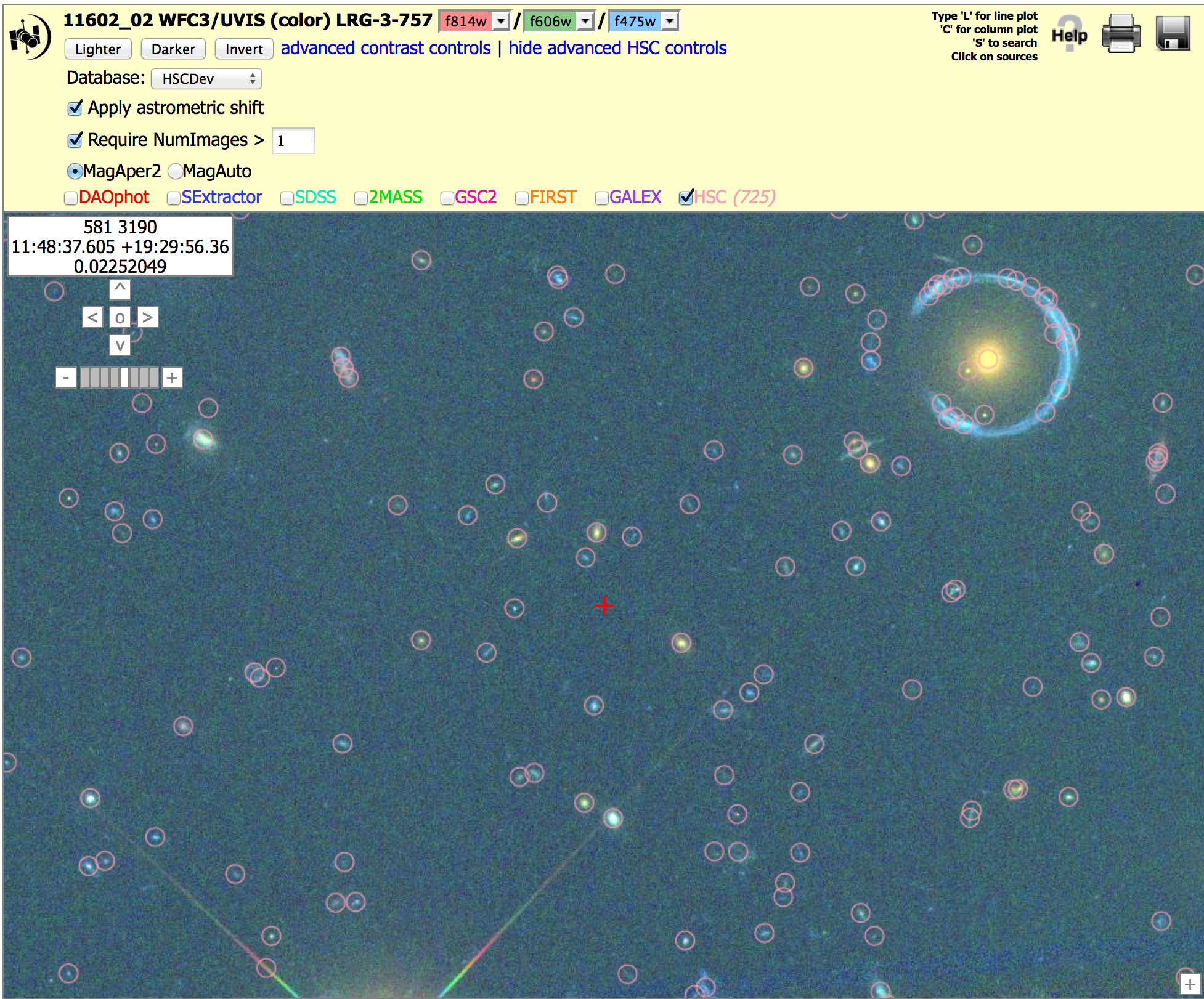
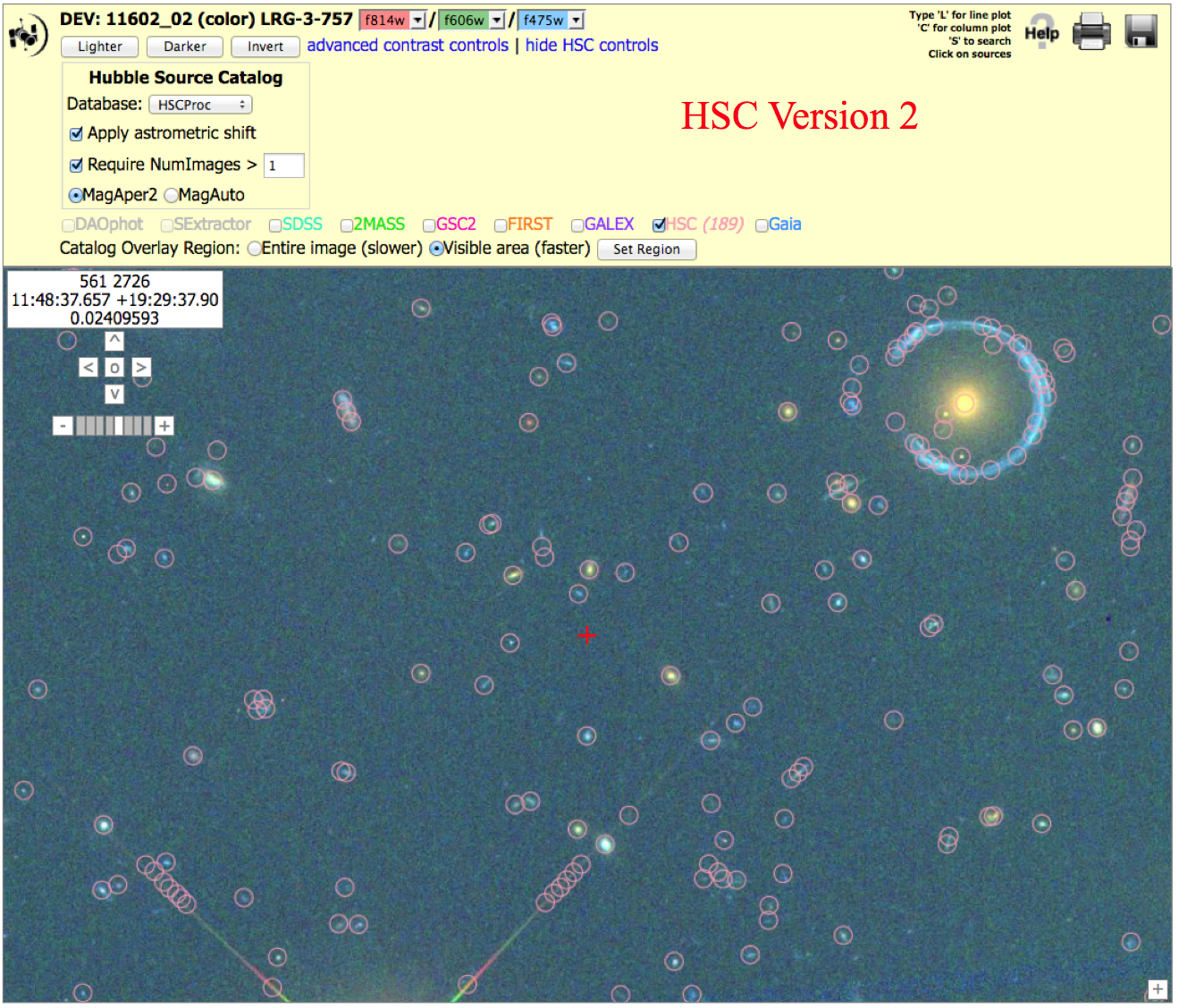
Gravitational Lens: WFC3/UVIS, (11602_02), N > 1 version To get the image below, click on "Advanced HSC controls", then check the box for "Require NumImages > 1", then click on HSC.
Note the presence of artifacts along the outer part of the diffraction spikes in the version 2 image. This is primarily due to going deeper for the ACS images. It is often possible to remove these by using the appropriate value of the NumImages criteria.
Also note that there are more sources measured around the gravitational ring, again resulting from the fact that the ACS images go deeper in version 2.
Mixed examples:
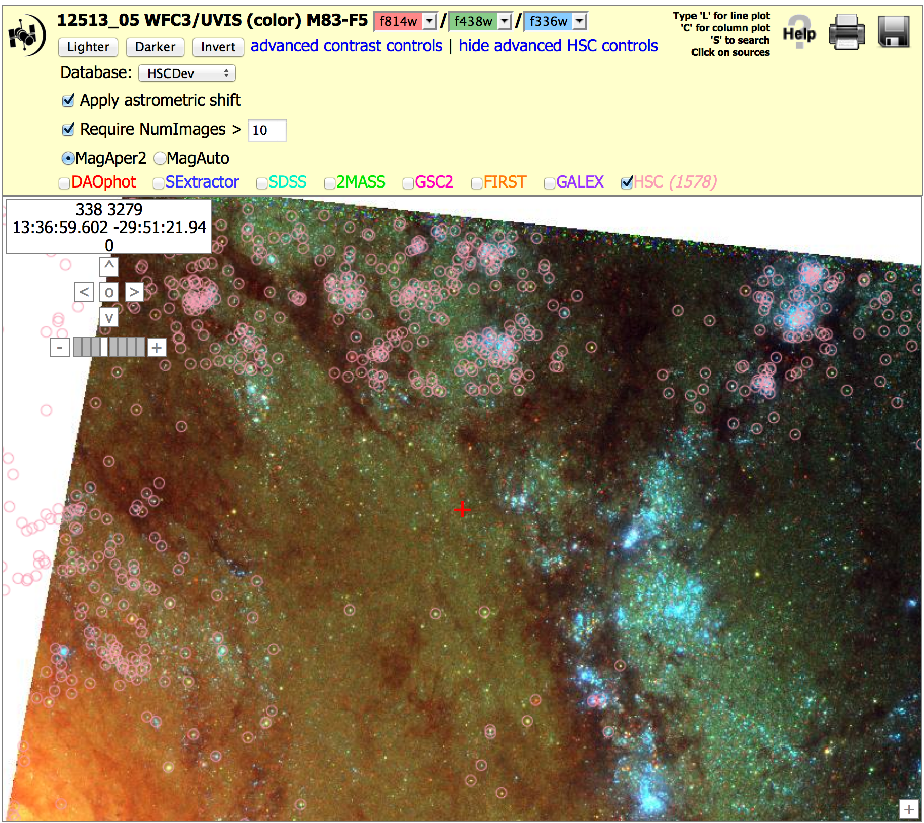
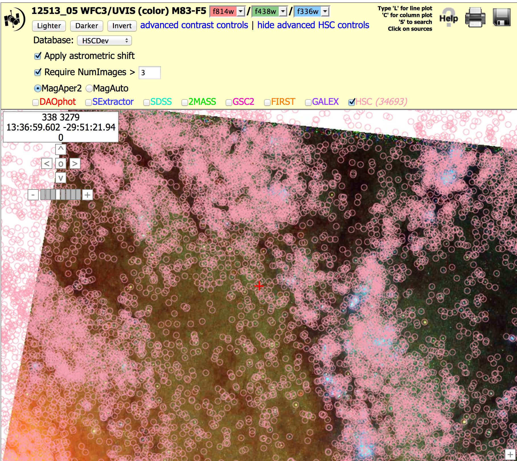
Nearby Galaxy WFC3/UVIS, (12513_05), N > 10 and 3 versions. To get the image below, click on "Advanced HSC controls", then check the box for "Require NumImages > 10", then click on HSC. Repeat this with "Require NumImages > 3"
This shows an example where a poor choice of NumImage > 10 can result in a very nonuniform catalog, while NumImages > 3 results in a more uniform catalog. Because of the strong sensitivity to the choice of NumImages, this is considered a mixed quality catalog.
NOTE: These figures are from version 1.
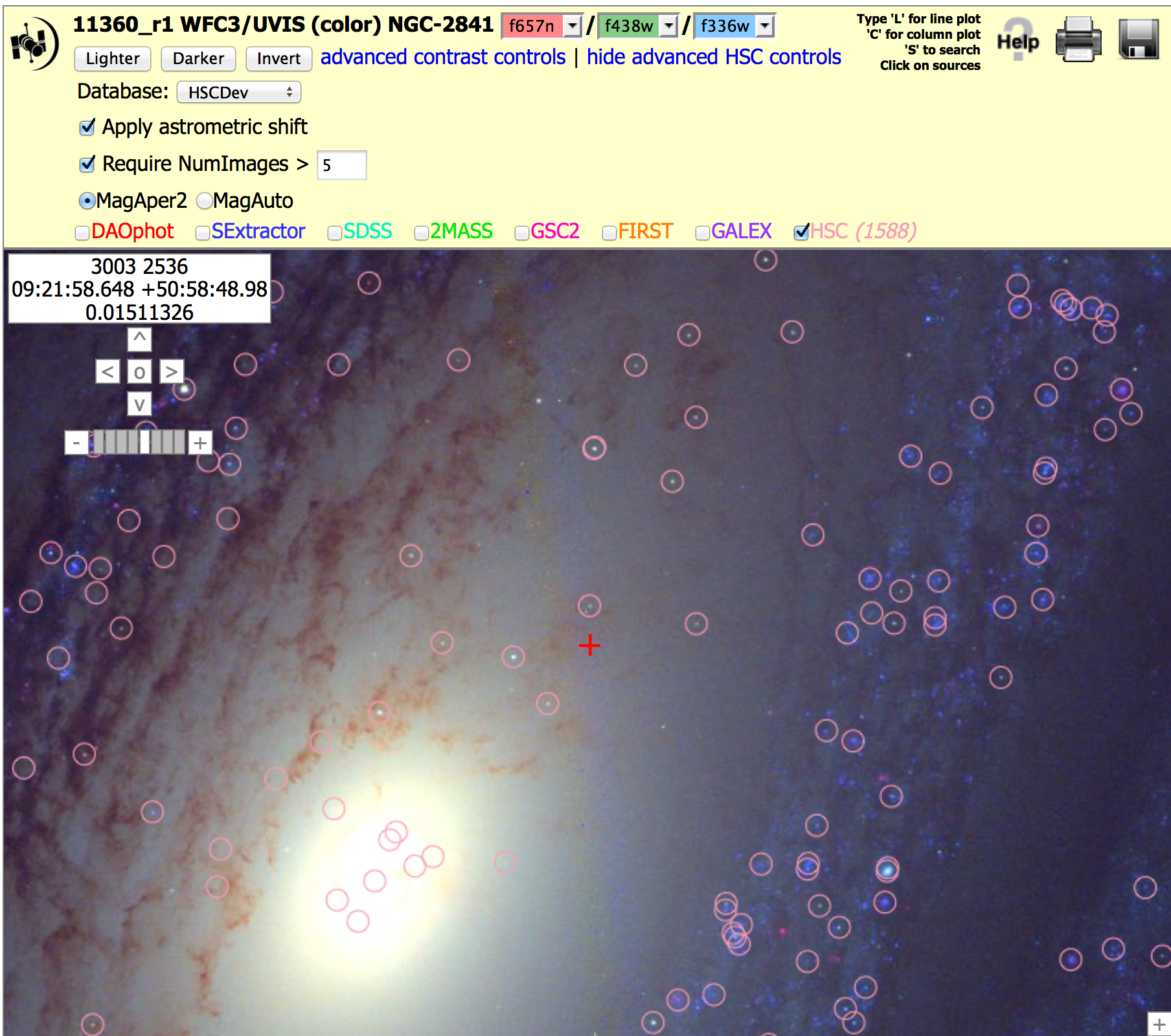
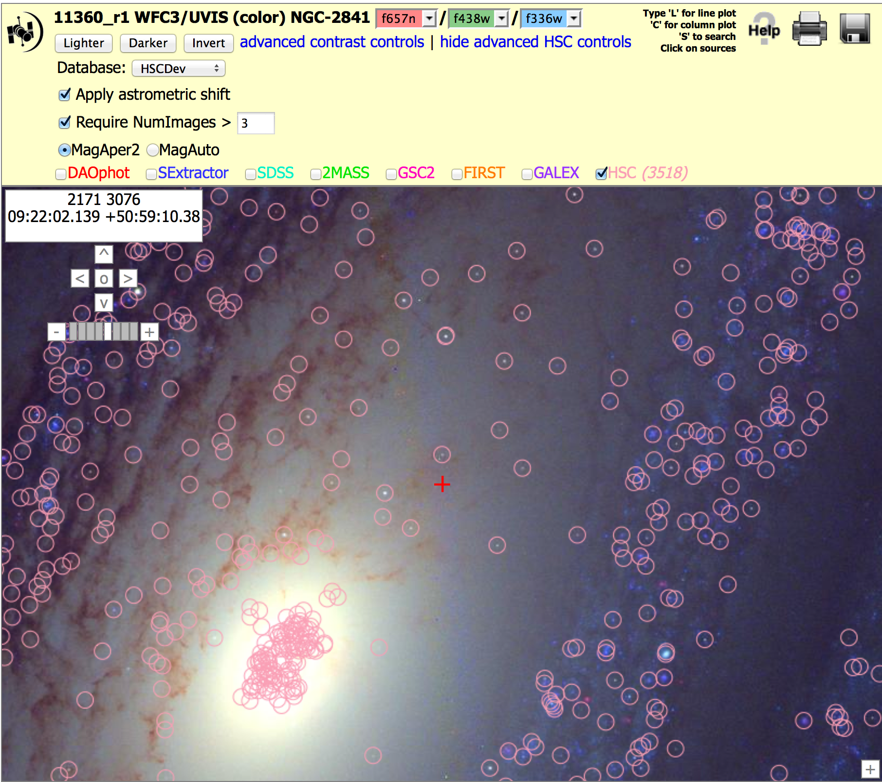
Nearby Galaxy WFC3/UVIS, (11360_r1), N > 3 and 5 versions. To get the image below, click on "Advanced HSC controls", then check the box for "Require NumImages > 3", then click on HSC. Repeat this with "Require NumImages > 5"
This shows an example where a poor choice of NumImage > 3 results in a number of false sources near the nucleus. While NumImages > 5 fixes most of this problem, it also results in the loss of many real sources. For this reason we consider this a mixed quality catalog.
NOTE: These figures are from version 1.
Bad Examples:
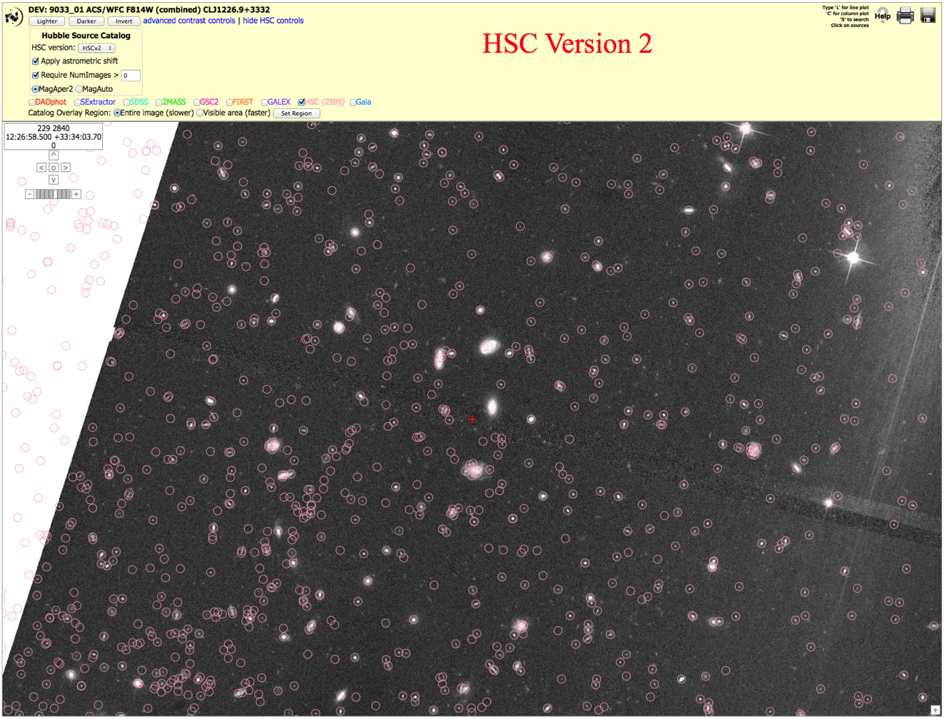
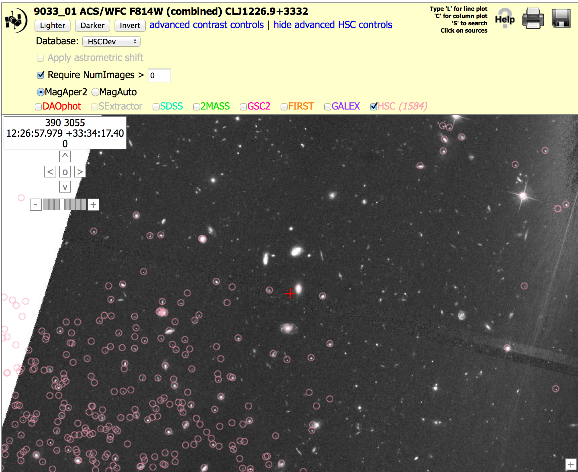
Field of Galaxies: ACS (9033_01), N > 0 version. To get the image below, click on "Advanced HSC controls", then check the box for "Require NumImages > 0", then click on HSC.
In version 1, the problem was that no Source Extractor source list was produced by the HLA, and hence the obvious galaxies in the center of this field are missing from the HSC. This can be seen by the fact that the SExtractor check box is greyed out. There are many reasons why a source list might be missing in the HLA. In this case it is probably because there is an extremely bright star just to the right of this field,
However, note that this problem has now been fixed in version 2, and so this region has changed from a Bad to a Good example !
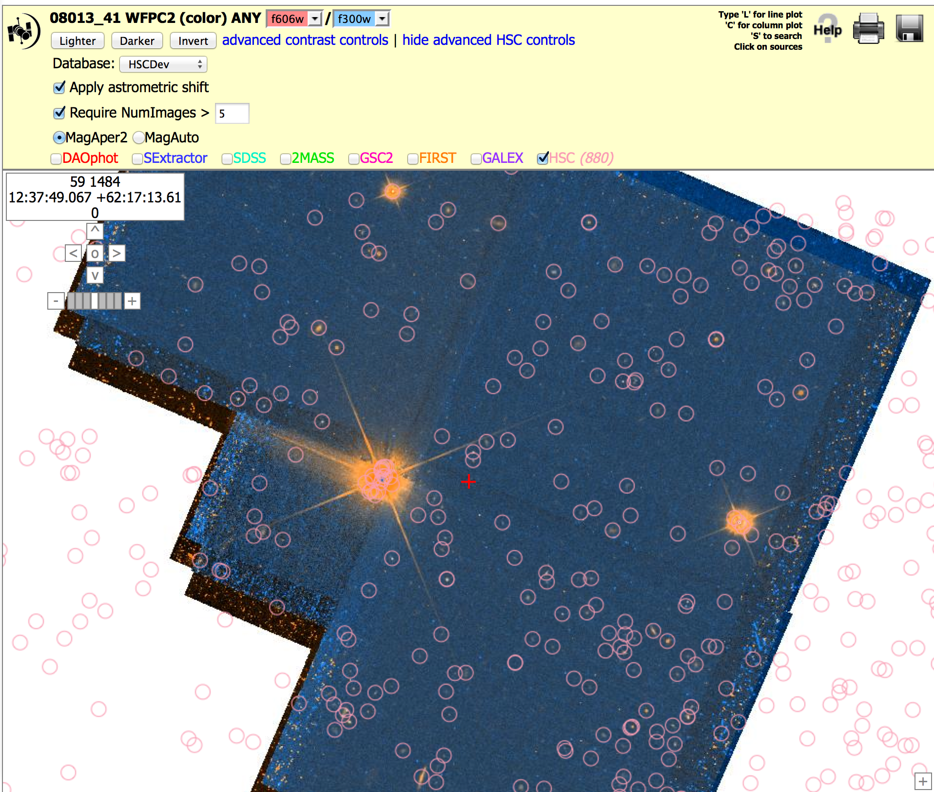
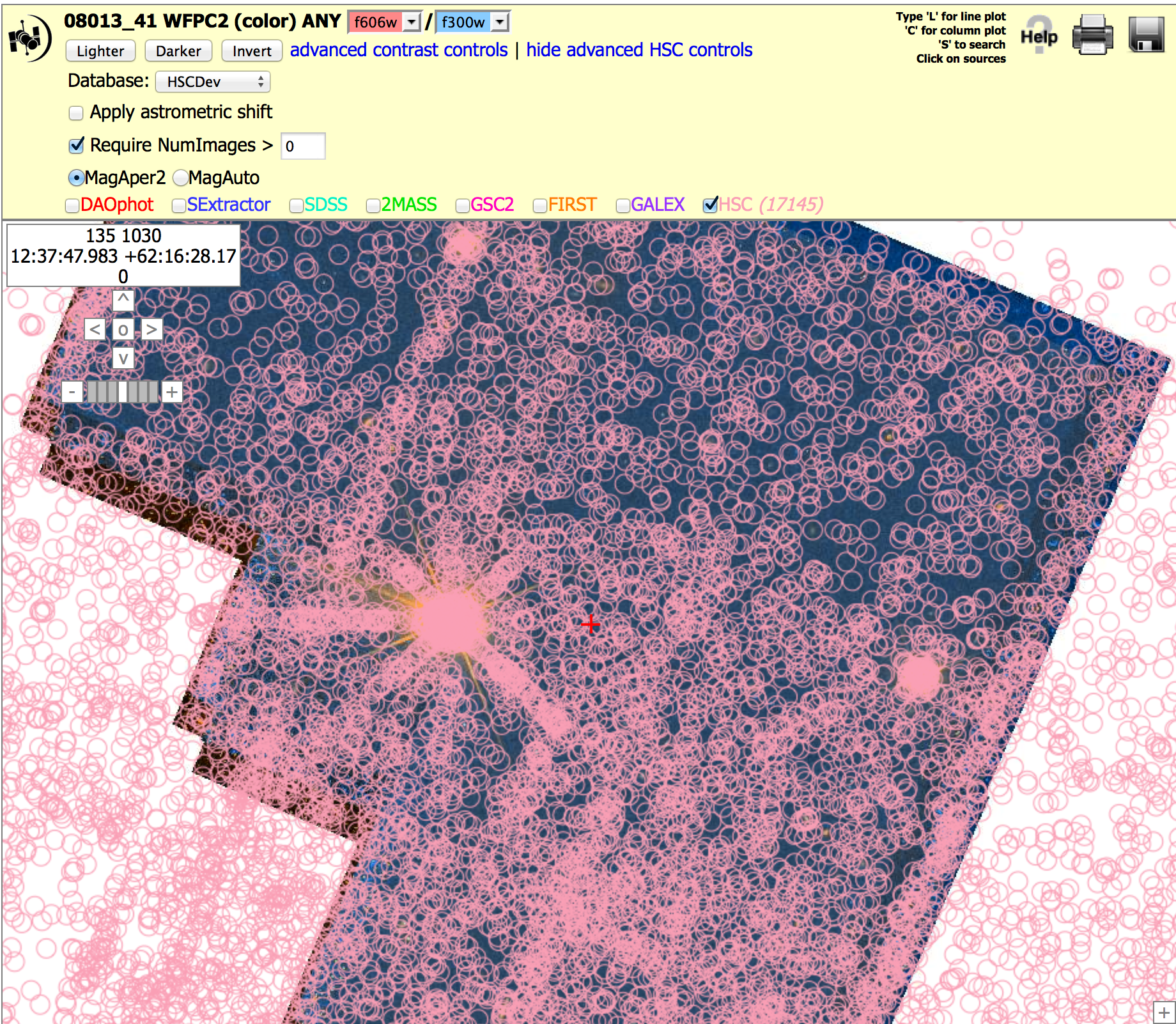
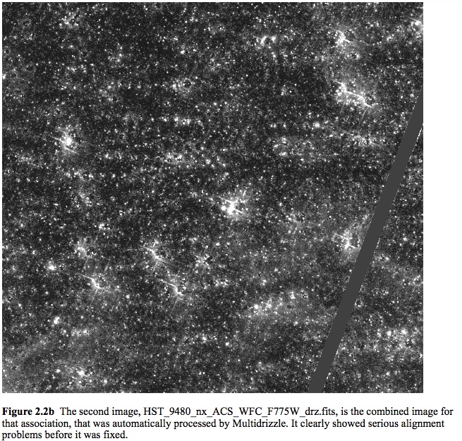
Starfield: WFPC2 (8013_41), N > 0 and 5 versions. To get the image below, click on "Advanced HSC controls", then check the box for "Require NumImages > 0", then click on HSC. Repeat this with "Require NumImages > 5".
This shows a field with a large number of artifacts in a WFPC2 field when using NumImages > 0, both because of the bright stars in the field and various edge effects. While using NumImages > 5 removes many of these artifacts, it is not possible to remove all of them without also removing many of the real sources.
NOTE: These figures are from version 1. Version 2 looks fairly similar since the WFPC2 images and source lists have not been redone.
-
What are the primary "known problems" with HSC Version 2?
Known Problem # 1 - Artifacts around bright stars and along diffraction spikes
These often appear to be more prevalent in version 2 compared to version 1, for example near the ends of the diffraction spikes in the image of the
gravitational lens (11602_02) shown here.
This is primarily due to going
deeper for the ACS images in version 2. It is generally possible to remove these by using the appropriate value of the NumImages criteria.
Known Problem # 2 - "Doubling"
 There are occasionally cases where not all the detections of the same source are matched together into a single objects. In these cases, more than one match ID is assigned to the object, and two pink circles are generally seen at the highest magnification in the display, as shown by the yellow arrows in the example. Most of these are very faint objects, and the primary reason there are more in version 2 compared to version 1 is the deeper ACS source lists.
These "double objects" generally have very different numbers of images associated with the two circles. Hence, this problem can often be handled by using the appropriate value of NumImages to filter out one of the two circles. For example, using Numimages > 9 for this field removes essentially all of the doubling artifacts, at the expense of loosing the faintest 25 % of the objects (see figure on right).
Interestingly, while investigating the doubling artifact we found that some cases are due to the proper motion of the star ! These can generally be separated from cases where the doubling is due to poor matching by examining the range of dates of the observations for the two circles. An example of this is currently being written up as a use case which will be included in the future.Known Problem # 3 - Edge Effects
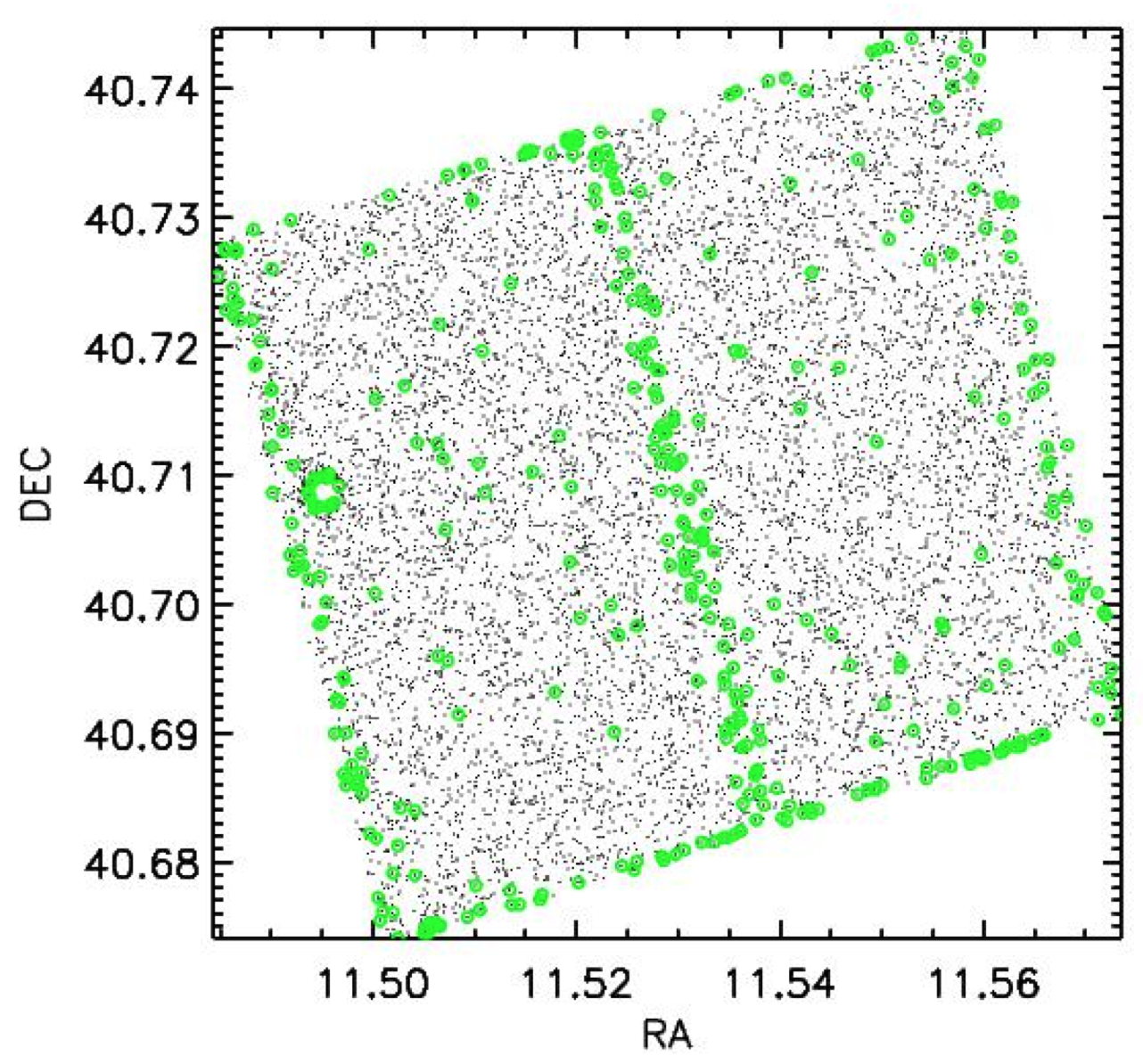 This figure is the byproduct of a project to find variable stars
by searching for outliers in photometric light curves. It reveals that the
photometry along the edges, and the chip gap between detectors, are
photometrically degraded in some images, with outliers that can be mistaken as
potential variables (i.e., the green points). While this complicates the ability to find
variables in these areas, the effect on mean photometric values is believed to be
relatively small in most cases. However, we caution users to be aware of this potential
issue by examining their results for potential edge effects.
The effect appears to be due to insufficient masking along the edges and gaps, but is still under
investigation.
A more detailed analysis of the effect on photometry will be included in this section in the future.
This figure is the byproduct of a project to find variable stars
by searching for outliers in photometric light curves. It reveals that the
photometry along the edges, and the chip gap between detectors, are
photometrically degraded in some images, with outliers that can be mistaken as
potential variables (i.e., the green points). While this complicates the ability to find
variables in these areas, the effect on mean photometric values is believed to be
relatively small in most cases. However, we caution users to be aware of this potential
issue by examining their results for potential edge effects.
The effect appears to be due to insufficient masking along the edges and gaps, but is still under
investigation.
A more detailed analysis of the effect on photometry will be included in this section in the future.
One method to minimize edge effects that often works is to restrict your sample to sources with larger values of NumImages, as shown in the discussion of the WFPC2 image for proposal-ID = 8013 in the Bad Examples section.
This effect was discovered during the development of the Hubble Catalogue of Variables an ESA-funded project under the direction of Alceste Bonanos at the National Observatory of Athens. We thank Ming Yang for discovering this effect and sending us the graphic.Known Problem # 4 - PC and WFC objects are combined for the WFPC2
Aperture magnitudes for objects on the PC (Planetary Camera) portion of the WFPC2 differ (typically by 0.2 to 0.3 magnitudes) when compared to the same object when it is on the WF (Wide Field) portion of the WFPC2, resulting in additional scatter for the WFPC2 data. This is caused by a variety of reasons including: 1) the pixel scale on the PC is half the size of the WF - while resampling adjusts for this to some degree, it does not fully compensate, 2) Charge Transfer Efficiency loss (CTE) is much higher on the PC due to the lower flux in the smaller pixels. In V2. Information about which chip the object is found on is stored in a table (named WFPC2PCFrac) that is available via CASJOBS. However, this information is not currently used when computing the normalized concentration index (CI) or magnitudes of sources in the summary form.Known Problem # 5 - Misaligned exposures within a visit.
 When combining images, the HLA assumes that exposures within a visit
are well aligned. This is generally a good assumption, but
occasionally is not true, especially when combining the observations
from one filter with another. This can result in "smeared" images, bad
photometry (because a position between the offset sources is
measured), and an abnormal Concentration Index.
When combining images, the HLA assumes that exposures within a visit
are well aligned. This is generally a good assumption, but
occasionally is not true, especially when combining the observations
from one filter with another. This can result in "smeared" images, bad
photometry (because a position between the offset sources is
measured), and an abnormal Concentration Index.
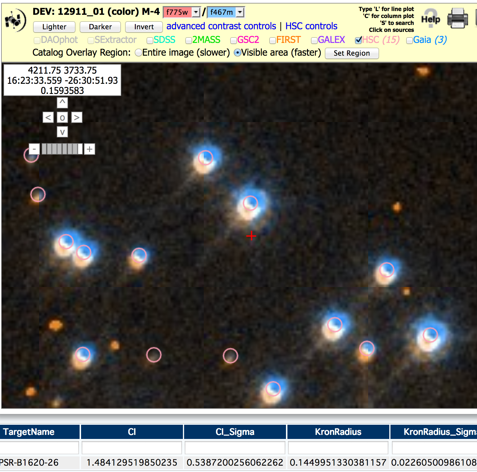
This figure shows an example resulting from a combination of WFC3/UVIS F775W and F467M observations in M4. By using the color image (enter level = 4 in the inventory column in the HLA) you can clearly see the offset between the blue (F467M) and red (F775) observations. In addition, the positions are between the two color images, the normalized concentration index (CI) is much larger than it should be for a star (i.e 1.48 rather than about 1.0), and the photometric sigma values in the two filters (not shown) are about 0.12 mag, much higher than the few hundreds of a magnitude that would be expected for a bright star.
In the future, this problem will be fixed by using the tweakreg feature in the astrodrizzle program.Known Problem # 6 - CTE loss corrections are made for WFPC2 and ACS, but not yet for WFC3/UVIS.
Corrections for Charge Transfer Efficiency (CTE) loss are made for WFPC2 based on the Dolphin (2009) formula. Corrections for CTE loss on the ACS/WFC are made by using images corrected using a pixel-to-pixel approach to CTE correction developed by Anderson & Bedin (2010) and incorporated into the HST calibration pipeline for ACS. Similar corrections have NOT been made for the WFC3 yet but are scheduled to be incorporated into the pipeline in the near future.
FAQ - About Images and Matches
-
How are HLA images and source lists constructed?
The Hubble Source Catalog (HSC) is based on HLA Source Extractor (Bertin & Arnouts 1996) source lists. To build these source lists, the HLA first constructs a "white light" or "detection" image by combining the different filter observations within each visit for each detector. This filter-combined drizzled image provides added depth. Source Extractor is run on the white light detection image to identify each source and determine its position.
Next, the combined drizzled image for each filter used in the detection image is checked for sources at the positions indicated by the finding algorithm in Source Extractor. If a valid source (flags less than 5) - is detected at a given position then its properties are entered into the HLA source list appropriate for the visit, detector, and filter. (See HLA Source List FAQ for a definition of the flagging system for HLA source lists. These are defined as level 0 detections, and are reported in the HSC Detailed Search Form to have a value of Det = Y.
Sources that are found in the white light detection image, but not in a particular filter used to make the white light image, are regarded as "filter-based nondetections". These can be examined by asking for level = 1 under the Detection Options on the HSC Detailed Search form.
It is also possible to use the Detection Option in the HSC Detailed Search Form to retrieve Level = 2. This Includes detections, filter-based nondetections, and visit-based nondetections. Visit-based nondetections are cases where an image overlaps with the specified positional search constraints, but no sources are detected there. Visit-level nondetections have a Det value of N and no assigned MatchID value when viewing the HSC Detailed Search Form.
More details about how HLA images are constructed can be found at the HLA Images FAQ . More details about how HLA source lists are constructed can be found at the HLA Source List FAQ.
A general outline of the entire process of making the HSC is available in section 3.1 of (Whitmore et al. 2016) . -
How are "matches" defined in the HSC? What is the algorithm that combines the sources?
The source detections (and nondetections) that correspond to the same physical object (as determined by the algorithms defined in Budavari & Lubow 2012) are given a unique MatchID number and an associated match position (MatchRA, MatchDec). Each member of the match, including nondetections, also has an assigned MemID value and a source position (SourceRA, SourceDec). As part of the matching process, astrometric corrections are made to overlapping images. Each source detection and nondetection has a separation distance, D (small d in the plots below), from the match position.
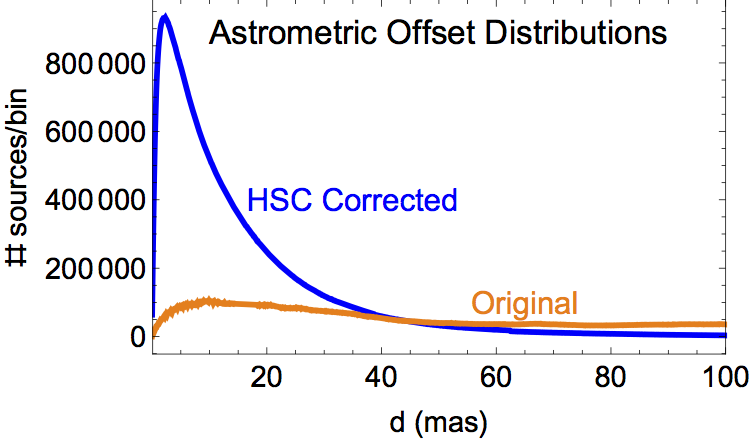
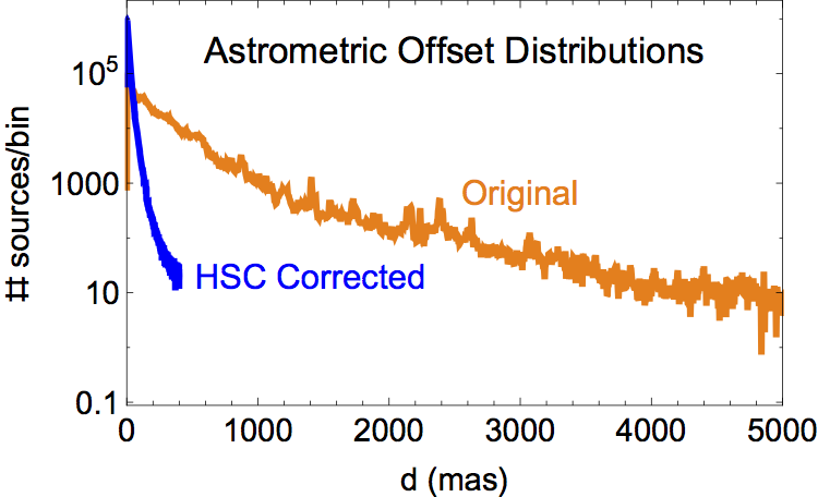
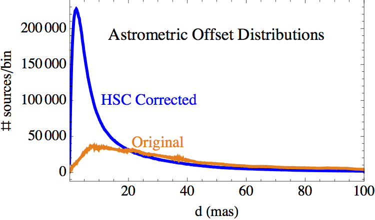
The two plots show (in blue) the distribution of the relative astrometric errors in version 2 of the HSC corrected astrometry, as measured by the positional offsets of the sources contributing to multi-visit matches from their match positions. Plotted in orange are the corresponding distributions of astrometric errors based on the original HST image astrometry. The areas under the blue and orange curves in the left plot should be the same, but are not due to the long tail in the orange curve that extends beyond the limits of the plot.
The left plot is on a much smaller distance scale than the right plot. Furthermore, the right plot has a logarithmic vertical scale. In version 2, the peak (mode) of the HSC corrected astrometric error distribution is 2.3 mas, while the median offset is about 10 mas. The original (current HST) astrometry has corresponding values of 6.8 mas and 160 mas, respectively. To summarize, the relative astrometric error distribution in the original HST images has a long tail that has been greatly reduced by the HSC corrections. -
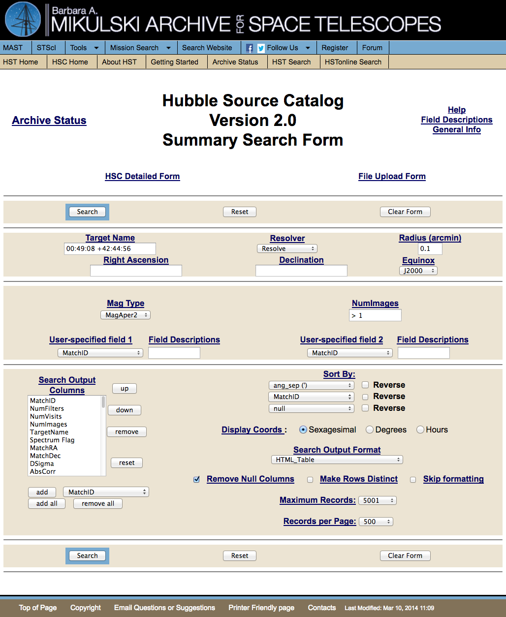
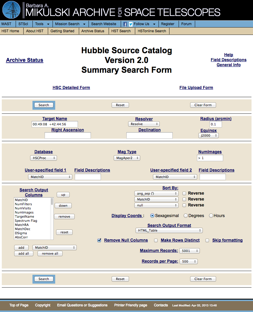
What is the HSC Detailed Search Form ?
NOTE: The plots shown in this section are from version 1, and will be replaced with figures from version 2 when they are available.
Although the primary way to access the HSC is through the MAST Discovery Portal, as discussed in the next section, we begin with a look at the HSC Detailed and Summary Search Forms, since it helps clarify what we mean by a match in the HSC.
Here is a portion of some output from the HSC Detailed Form showing the matches for MatchID 22214697. Each source detection (i.e., SourceID) and nondetection (Det = N) has some separation distance, D, from the match position. The Dsigma value is the standard deviation of the D values, and is also reported in the HSC Summary Search Form.
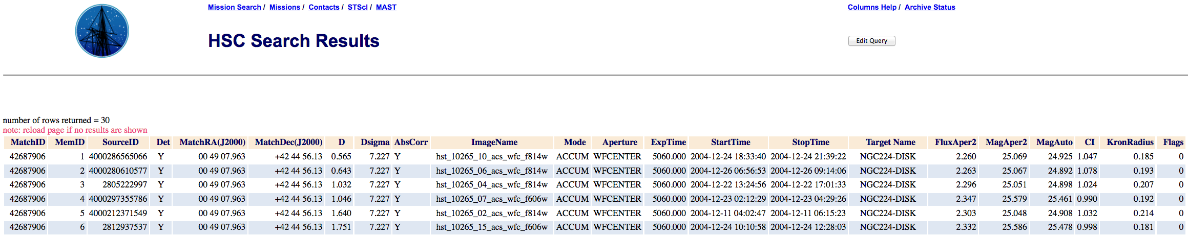
...

Many of the detections in the Detailed Search Form are in matches that involve a single visit and detector. These cases have D=0 and Dsigma=0.
-
What is the HSC Summary Search Form? What are some of the primary columns?
The HSC Summary Search Form includes results for all detections for a given match on a single row. The magnitudes for different visits are averaged together, along with a variety of other information.
Example Output - Left portion:
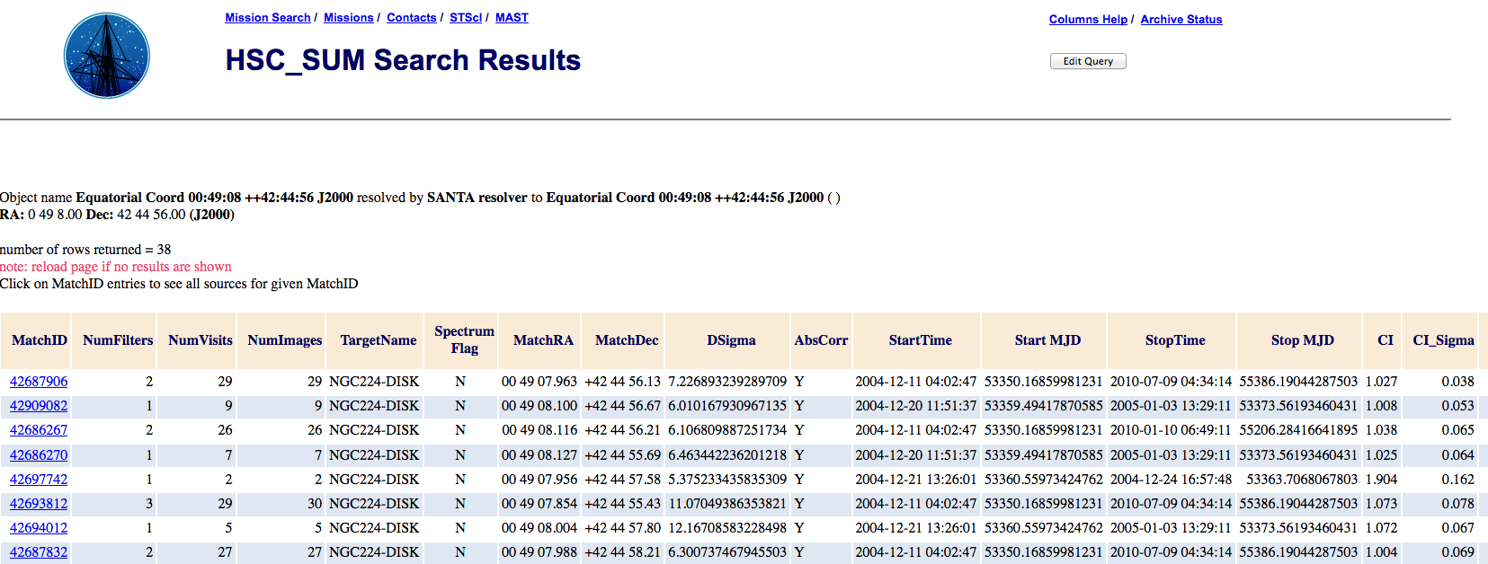
Example Output - Right portion:
More information about the individual detections that went into a given match can be obtained by searching the Detailed Search Form for the appropriate MatchID value by clicking on the blue MatchID value in the first column of the Summary Search Form.
For a short description of each column, click on "Field Descriptions" in the upper right of the HSC Summary Search Form. Slightly more detailed descriptions for some of the key columns (not already discussed for the Detailed Search Form above) are included below. For even more detailed information the HLA FAQ - About Source Lists is available.
NumImages = Number of separate images in a match. Often used to filter out artifacts (e.g., NumImages > 1 will remove most cosmic rays).
 Spectrum Flag =
Is there a matching COS, FOS, or GHRS spectral observation associated with this source? See "What are the columns in the spectral results page?" for details.
Spectrum Flag =
Is there a matching COS, FOS, or GHRS spectral observation associated with this source? See "What are the columns in the spectral results page?" for details.
AbsCor = Was it possible to correct the absolute astrometry (Y/N) by matching with Pan-STARRS, SDSS, or 2MASS.
Start and Stop MJD = Modified Julian Date (MJD) for the earliest and latest image in the match.
CI (Normalized Concentration Index) =
Mean value of the "Normalized" Concentration Index, defined as the
difference in aperture magnitudes using the small aperture (i.e., MagAper1)
and large aperture (MagAper2). Note that CI was not normalized in version 1.
CI can often be used to help
separate stars from extended sources.
CI_Sigma = Standard Deviation in the CI values for this MatchID.
KronRadius = Kron Radius in arcsec from the Source Extractor algorithm. IMPORTANT NOTE: The minimum value (i.e., for point sources) is 3.5 pixels, which translates to 0.14 arcsec for WFC3/UVIS, 0.175 arcsec for ACS/WFC, 0.315 arcsec for WFC3/IR, and 0.35 arcsec for WFPC2. Watch for a pileup of measurements at these values that are due to this limit rather than reflecting a real peak.
KronRadius_Sigma = Standard Deviation in the CI values for this MatchID.
Extinction = E(B-V) from Schlegel (1998).
Instrument_Filter = Mean magnitude for all detections in the match, grouped by instrument (A = ACS, W2 = WFPC2, W3 = WFC3) and filter combination. The order is from short to long wavelengths. The values are in the ABmag system. The default is to provide MagAper2 values (i.e.,aperture photometry using the large aperture - see CI description above), but you can also request MagAuto (using the Source Extractor algorithm) values if you are more interested in extended sources.
In HSC version 2.1 (January 2017), tables have been made available via HSC CASJOBS providing MEDIAN rather than MEAN values for magnitudes from the summary form (i.e., table SumMagAper2Med for magaper2 values and table SumMagAutoMed for magauto values). This provides more reliable values for cases where there are large photometric deviations for some of the individual measurements. In general, use of this table will introduce only very small differences compare to the mean values. Here are details on how to access the median tables.
Instrument_Filter_Sigma = Standard Deviation around mean magnitude for this Instrument_Filter combination.
Instrument_Filter_N = Number of measurements that went into the determination of mean magnitude for this Instrument_Filter combination.
Ang Sep(') = Angular Separation for this match from the position used to make the search.
-
-
-
-
-
-
How do I find the HSC photometric data corresponding to an individual object?
If you click on the Load Detailed
-
-
How can I cross match objects between Version 1 and Version 2?
There may be circumstances when a researcher has a list of objects they were working on from HSC version 1 but would now like to identify their counterparts in Version 2. This can be done using a table called xMatchV1 which is available via HSC CASJOBS.
After logging into HSC CASJOBS (see HSC Use Case #2 if you are not familiar with CASJOBS), click on MyDB and then set the context to HSC2v2. Under Tables you will find the file xMatchV1. Click on that to see the help file. Try running the example as a query.
Here is a short script showing how to do a match for a specific region of the sky around M83.
select s2.MatchRA, s2.MatchDec, x.MatchID, x.MatchID1, d=dbo.fDistanceArcMinEq(s1.MatchRA, s1.MatchDec, s2.MatchRA, s2.MatchDec)*60.0*1000, Rank
from xmatchv1 x join hscv1.SumPropMagAper2Cat s1 on x.MatchID1=s1.MatchID
join SumPropMagAper2Cat s2 on x.MatchID=s2.MatchID
where s1.MatchRA > 204.252 and s1.MatchRA < 204.256 and s1.MatchDEC > -29.867 and s1.MatchDEC < -29.863
and x.Rank < 2 and x.DistArcSec < 0.1
 Note that this script assumes:
1. Only the nearest source should be listed (i.e., x.rank < 2, there may be circumstances when you relax this to look for other nearby sources.)
2. The largest value of the distance between the V1 and V2 source should be 0.1 arcsec (i.e., 100 mas (i.e., xDistArcSec < 0.1)
These two parameters (and others such as the RA and DEC of course) can be modified in the script if different values are wanted.
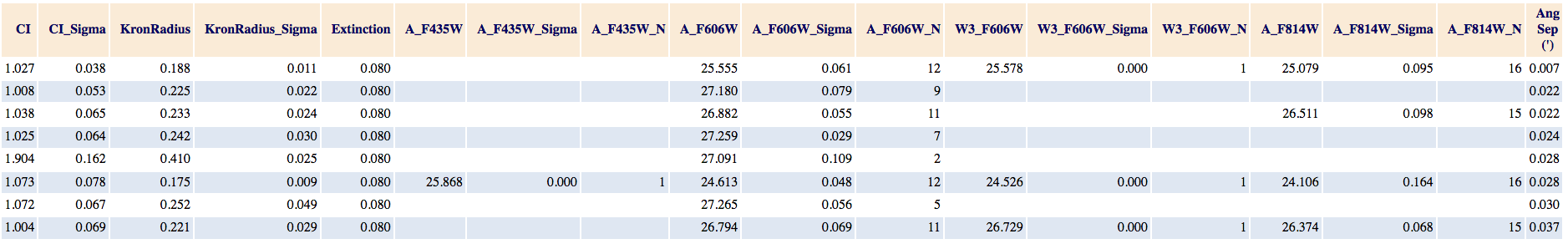
The output can be saved as a file and then read into the Discovery Portal to examine the quality of the cross matching. Modifications (e.g., a different upper limit in D) can also be made in the Discovery Portal (see the graphic on the right for an example) and then saved in a file, or the user can go back to the HSC CASJOB query and make modifications there if they prefer.
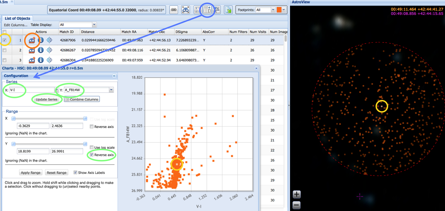
In HSC version 2, two important improvements have been made to the Discovery Portal.
1) The maximum number of HSC sources it can upload has been increased from 10,000 to 50,000,
2) The Discovery Portal can now access both aperture magnitudes (i.e., MagAper2) and estimates of total magnitudes (i.e., using the MagAuto algorithm in Source Extractor).
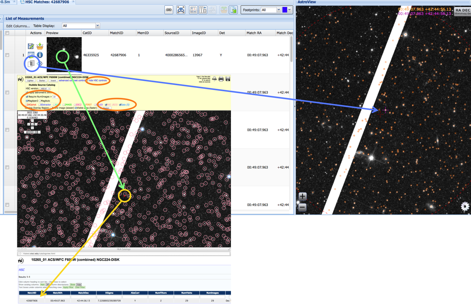
Here we show an example (from HSC Use Case # 1 of using the Discovery Portal to make a color-magnitude diagram, highlighting a specific object (yellow) and showing its location in the image, its values in the table, and its position in the plot.
NOTE: Both HSC versions 1 and 2 are available using the cross-match capabilities of the Discovery Portal. However, only version 2 is available via the "Select a collection" box for the rest of the capabilities. Both versions 1 and 2 ARE available via CASJOBS and the HSC Home Page and Search forms.
-
FAQ's specific to the Discovery Portal.
Question: I looked at the HLA Interactive Display and saw that there were 100,000 objects in the HSC for a specifc image. Why does the Discovery Portal (DP) query only return 50,000?
Answer: 50,000 is the maximum number of records currently supported for query results in the Discovery Portal. Larger queries can be handled in the HSC CasJobs tool.
Question: Can I import my own catalog of objects into the DP?
Answer: Yes, using the "Upload Target List" button just below the "Select a collection" box (i.e., the icon).
Question: Where is the plot icon you mention in the use case? I don't see it on the screen.
Answer: Depending on the size of the box with the target position (entering a target position generally makes the box big while entering a target name does not), the AstroView window can COVER UP the icon. By grabbing the side of the AstroView window and dragging to the right, you can shrink the window and reveal the row of icons.
 Question:
Can I overlay the HSC on HST images?
Question:
Can I overlay the HSC on HST images?
Answer: Yes. After doing your query, click on the icon under
Actions (Load Detailed Results)
. This will show you the
details for a particular MatchID, including cutouts for all the HST
images that went into this match. If you then click on the
icon under
Actions (Load Detailed Results)
. This will show you the
details for a particular MatchID, including cutouts for all the HST
images that went into this match. If you then click on the  icon under Action (Toggle Overlay Image) (blue circle in the image
- see Use Case # 1), the HST
image will be displayed over the DSS image in AstroView
icon under Action (Toggle Overlay Image) (blue circle in the image
- see Use Case # 1), the HST
image will be displayed over the DSS image in AstroView
Question: Can I bring up the HLA interactive viewer from the DP?
Answer: Yes. After doing your query, click on the first
icon under
Actions (Load Detailed Results). This will show you the
details for a particular MatchID, including cutouts for all the HST images that went into this match. If you click on the
cutout (green circle in the image - see Use Case # 1)
, the HLA interactive viewer will come up.
Question: Can I change the contrast control in the AstroView window?
Answer: Not at this time. The HLA Interactive Display, discussed above, can be used for this.
Question: Can I center the field on a selected target?
Answer: Yes, click on the bulls-eye icon for the target of interest.
-
How can I use CasJobs to access the HSC?
The primary purpose of the HSC Catalog Archive Server Jobs System (CasJobs) is to permit large queries, phrased in the Structured Query Language (SQL), to be run in a batch queue. CasJobs was originally developed by the Johns Hopkins University/Sloan Digital Sky Survey (JHU/SDSS) team. With their permission, MAST has used version 3.5.16 of CasJobs to construct three CasJobs-based tools for GALEX, Kepler, and the HSC.
 While HSC CasJobs does not
have the limitations of only including a
small subsample of the HSC (i.e., 50,000 objects), as is the
case for the MAST Discovery Portal, it
also does not have the wide variety of
graphic tools available in the Discovery
Portal. Hence the two systems are
complementary.
While HSC CasJobs does not
have the limitations of only including a
small subsample of the HSC (i.e., 50,000 objects), as is the
case for the MAST Discovery Portal, it
also does not have the wide variety of
graphic tools available in the Discovery
Portal. Hence the two systems are
complementary.
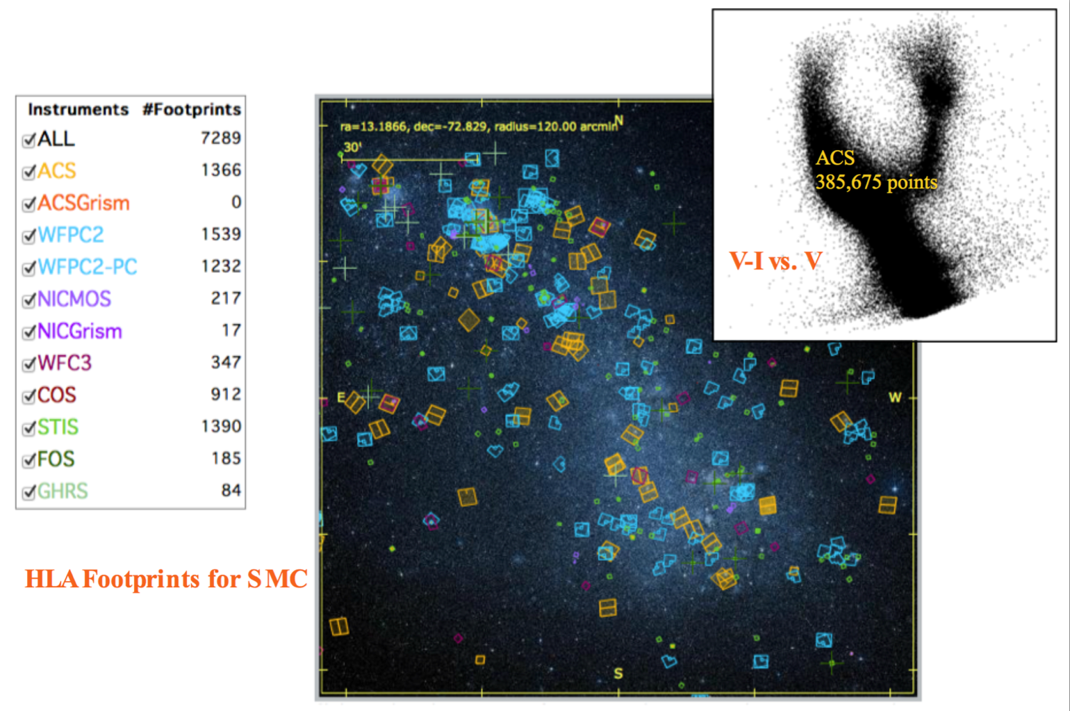
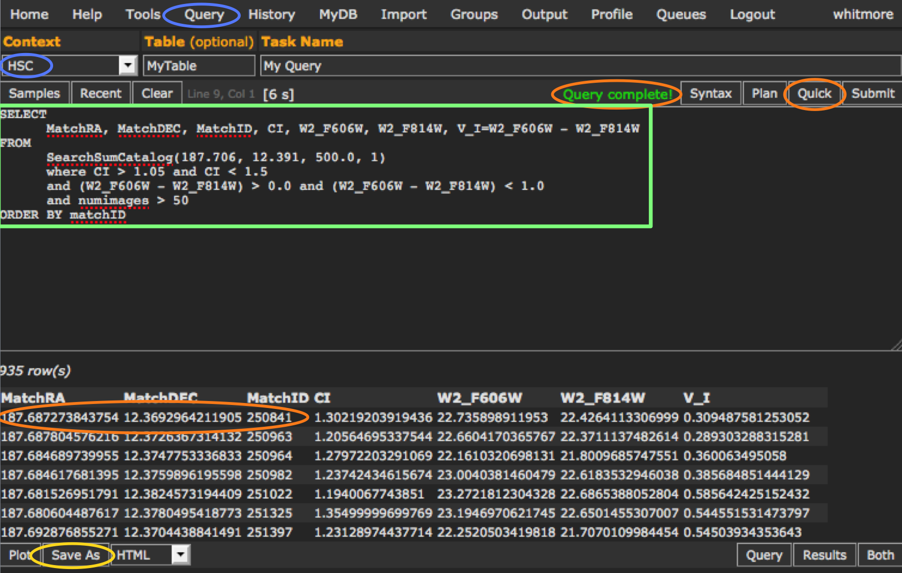
This figure (from HSC Use Case # 2) provides a demonstration of the speed and power of the HSC CasJobs interface. Starting from scratch, imagine how long it would take to construct a color-magnitude diagram for all Hubble observations of the Small Magellanic Cloud (SMC). A search of the HLA shows 7,289 observations in this region, 1366 of them with ACS. With HSC CasJobs, a color-magnitude can be made for ACS data in less than two minutes.
Casjobs also provides a personal database (i.e. myDB) facility where you can store output from your queries and save stored procedures and functions. This powerful aspect of Casjobs can also be used as a group sharing facility with your collaborators. -
FAQ's specific to the CasJobs.
Question: Why does my query give me an error saying that the function I was using (e.g. SearchSumCatalog) is an invalid object name?
Answer: This error usually indicates that the context is set incorrectly. Check that the context says HSC and not MyDB. This is probably the MOST FREQUENT PROBLEM people have with HSC CasJobs. (i.e., the blue oval under Context in the image - see use case # 2 for more details)
 Question:
I created an output catalog a while ago, and when I go to the
Output tab it is no longer there. What happened to it?
Question:
I created an output catalog a while ago, and when I go to the
Output tab it is no longer there. What happened to it?
Answer: There is a lifetime for output of 1 week.
Question: When I tried to plot my table, I got an error message saying that the input string was not in a correct format. What is wrong?
Answer: If there are any entries that have non-numeric values (such as NaN indicating no data), the plotting tool cannot handle them. The solution is to restrict your queries to only real numbers by adding a condition such as: A_F606W > 0 which will only include sources with measured values.
Question: What does 'Query results exceed memory limitations' mean?
Answer: This means the result of the query which you've submitted is greater than the memory buffer will allow. This message only applies to 'quick' queries; queries using 'submit' do not have any memory restrictions. The easiest thing to do is just use submit instead of quick.
Question: How do I see all the searches I have done?
Answer: The History page will show all the queries you have done, as well as summary information (submit date, returned rows, status). If you click on Info, you can see the exact query that executed, and resubmit the job if you like.
Question: How do I see all the results I have generated?
Answer: The MyDB page shows you all the tables you have generated. Clicking on the table name will show you the details of the table.
Question: How do I see all the available HSC tables, functions, and procedures?
Answer: Click on the MyDB at the top of the page, and then set the context to HSC. Clicking on the Views (currently empty), Tables, Functions, and Procedures will list the available material. Clicking on specific tables or functions will provide more information. (NOTE: When looking at functions, the default is to show the source code. To see the description instead, click on "Notes" near the top of the page.)
Question: Where are some example queries to run ?
Answer: Several of the HSC Use Cases have examples (e.g., Use Cases #2 and #5). Another good place to look is by clicking the Samples button after you hit the Query button (e.g., provides examples of cross matching and making histograms). There are also pointers to SDSS training materials on the left of the HSC HELP page.
Question: Where can I find the schema information for various HSC tables, functions and procedures (i.e., similar to the SDSS SkyServer Schema Browser)?
Answer: To get the schema for different HSC tables, function and procedures, first go to the top of the page and click on MyDB to bring up the database page. Next go to the drop down menu in the upper left and select HSC as the "context". Now click on one of the tables to see its schema information. To view schema for views, functions and procedures, click on the appropriate link below the context menu.
-
How can I use the HSC Home Page and Search Forms?
The HSC Summary and Detailed Search Forms, accessible from the HSC Home Page, provided the original access tool (e.g., for the Beta releases). While they may still be useful for certain very detailed searches, they have been largely superseded by the Discovery Portal and HSC CasJobs tools. The CasJobs tool can be used to issue the same queries used by the HSC Search Forms, as well as many other possible queries, but it requires SQL code.
There are two forms-based interfaces to the catalog that follow the
conventions of MAST. These are the
Summary Search Form, which allows users
to obtain mean magnitudes and other information with one row per
match; and the Detailed Search Form, that provides information about each
individual detections in a match.
Here are some examples of when it might be appropriate to use the HSC Search Forms rather than either the Discovery Portal or the HSC CasJobs.
-- Adding, deleting, or rearranging some of the columns on the HSC Summary Form. This is possible using the Output Columns on the HSC Summary Search Form.
-- Looking for non-detections. It is sometimes useful to have information about when an object is NOT found on an image. This is possible by changing the Detection Options on the HSC Detailed Form. See this link for a discussion of level 0, 1, and 2 detections.
-- Changing the format of the output from the HSC Summary or Detailed Search Forms. The HSC Search Forms have a wider variety of format options than the Discovery Portal of CasJobs. Examples are providing output coordinates in Sexagesimal, Degrees, or Hours; 17 different output formats including html, VOtables, comma-, tab-, space-, pipe-, or semicolon-separated, JSON, IRAF space-separated with-INDEFS, and excel_spreadsheets.
-
FAQ's specific to the HSC Home Page and Search Forms.
Question: Where can I find definitions of the columns in the HSC Summary or Detailed Search Forms?
Answer: For a short description of each column, click on "Field Descriptions" in the upper right of the Search Form. Slightly more detailed descriptions for some of the key columns are included here. For even more detailed information the HLA Source List FAQ is available.Question: Can a list of targets be used for a HSC search?
Answer: Yes - A list of targets can be searched using the "File Upload Form" button, which is located near the top right of either the HSC Summary or Detailed Search forms. The "Local File Name" box (or "Browse" pull-down menu) allows you to provide the name of a file listing the targets you would like to include in the search. A number of different format options for the input file are allowed, as defined in the target field definition portion of the form.FAQ - About Quality
-
What are specific limitations and artifacts that HSC users should be aware of?
NOTE: Unless otherwise noted, the graphics in this section are taken from version 1.
The Hubble Source Catalog is composed of visit-based, general-purpose source lists from the Hubble Legacy Archive (hla.stsci.edu) . While the catalog may be sufficient to accomplish the science goals for many projects, in other cases astronomers may need to make their own catalogs to achieve the optimal performance that is possible with the data (e.g., to go deeper). In addition, the Hubble observations are inherently different than large-field surveys such as SDSS, due to the pointed, small field-of-view nature of the observations, and the wide range of instruments, filters, and detectors. Here are some of the primary limitations that users should keep in mind when using the HSC .
LIMITATIONS:
Uniformity: Coverage can be very non-uniform (unlike surveys like SDSS), since a wide range of HST instruments, filters, and exposure times have been combined. We recommend that users pan out to see the full HSC field when using the Interactive Display in order to have a better feel for the uniformity of a particular dataset. Adjusting the value of NumImages used for the search can improve the uniformity in many cases. See image below for an example.
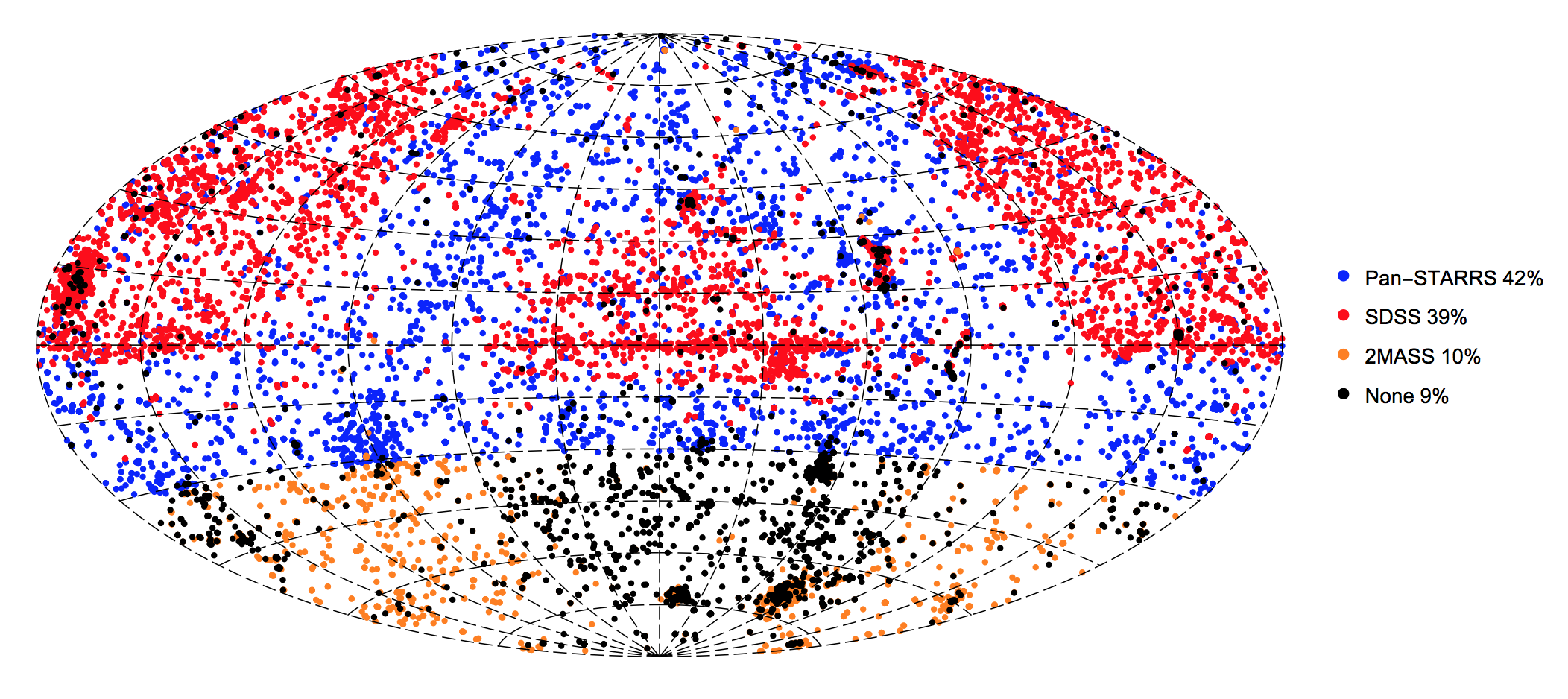
Astrometric Uniformity: In version 2, about 91% of HSC images have coverage in Pan-STARRS, SDSS, or 2MASS that permits absolute astrometric corrections of the images (i.e., AbsCor = Y) to a level of roughly 0.1 arcsec. See (Whitmore et al. 2016) for more details about astrometry, and to see the corresponding map for version 1. We note that in version 2 we changed the algorithm to use all three datasets, weighted by their goodness of fit. For the figure we show only the dataset with the best-fit value. This tends to weight SDSS more heavily than in version 1 .
Depth: The HSC does not go as deep as it is possible to go. This is due to a number of different reasons, ranging from using an early version of the WFPC2 catalogs (see "Five things you should know about the HSC" ), to the use of visit-based source lists rather than a deep mosaic image where a large number of images have been added together.
Completeness: The current generation of HLA WFPC2 Source Extractor source lists have problems finding sources in regions with high background. The ACS and WFC3 sources lists are much better in this regard. The next generation of WFPC2 sources lists will use the improved ACS and WFC3 algorithms, and will be incorporated into the HSC in the future.
Visit-based Source Lists: The use of visit-based, rather than deeper mosaic-based source lists, introduces a number of limitations. In particular, much fainter completeness limits, as discussed in Use Case # 1. Another important limitation imposed by this approach is that different source lists are created for each visit, hence a single, unique source list is not used. A more efficient method would be to build a single, very deep mosaic with all existing HST observations, and obtain a source list from this image. Measurements at each of these positions would then be made for all of the separate observations (i.e., "forced photometry"). This approach will be incorporated into the HSC in the future.
ARTIFACTS:
False Detections: Uncorrected cosmic rays are a common cause of blank sources. Such artifacts can be removed by requiring that the detection be based on more than one image. This constraint can be enforced by requiring NumImage > 1.
Another common cause of "false detections" is the attempt by the detection software to find large, diffuse sources. In some cases this is due to the algorithm being too aggressive when looking for these objects and finding noise. In other cases the objects are real, but not obvious unless observed with the right contrast stretch and field-of-view. It is not easy to filter out these potential artifacts without loosing real objects. One technique users might try is to use a size criteria (e.g., concentration index = CI) to distinguish real vs. false sources.
Doubling:
There are occasionally
cases where not all the detections of the same
source are matched together into a single
objects. In these cases, more than one match
ID is assigned to the object, and two pink
circles are generally seen at the highest
magnification in the display, as shown by the
yellow arrows in the example. Most of
these are very faint objects, and the primary
reason there are more in version 2 compared to
version 1 is the deeper ACS source lists.
These "double objects" generally have very different numbers of images associated with the two circles. Hence, this problem can often be handled by using the appropriate value of NumImages to filter out one of the two circles. For example, using Numimages > 9 for this field removes essentially all of the doubling artifacts, at the expense of loosing the faintest 25 % of the objects (see figure on right )Mismatched Sources: The HSC matching algorithm uses a friends-of-friends algorithm, together with a Bayesian method to break up long chains (see Budavari & Lubow 2012) to match detections from different images. In some cases the algorithm has been too aggressive and two very close, but physically separate objects, have been matched together. This is rare, however.
Bad Images: Images taken when Hubble has lost lock on guide stars (generally after an earth occultation) are the primary cause of bad images. We attempt to remove these images from the HLA, but occasionally a bad image is missed and a corresponding bad source list is generated. A document showing these and other examples of potential bad images can be found at HLA Images FAQ. If you come across what you believe is a bad image please inform us at archive@stsci.edu
-
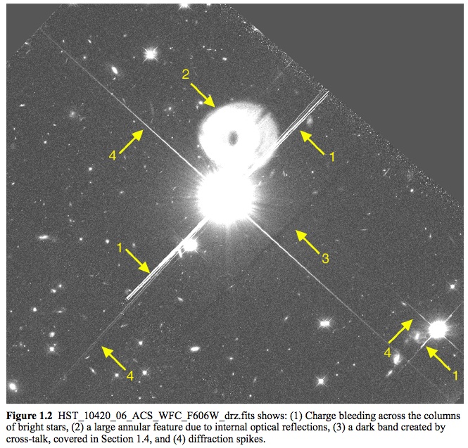
Is there a summary of known image anomalies?
Yes - HLA Images FAQ. Here is a figure from the document showing a variety of artifacts associated with very bright objects.
-
How good is the photometry for the HSC?
NOTE: This section is based on version 1 of the HSC, and more specifically, the studies performed for the (Whitmore et al. 2016) paper. Similar ongoing analysis of the version 2 database will be added to this section in the future.
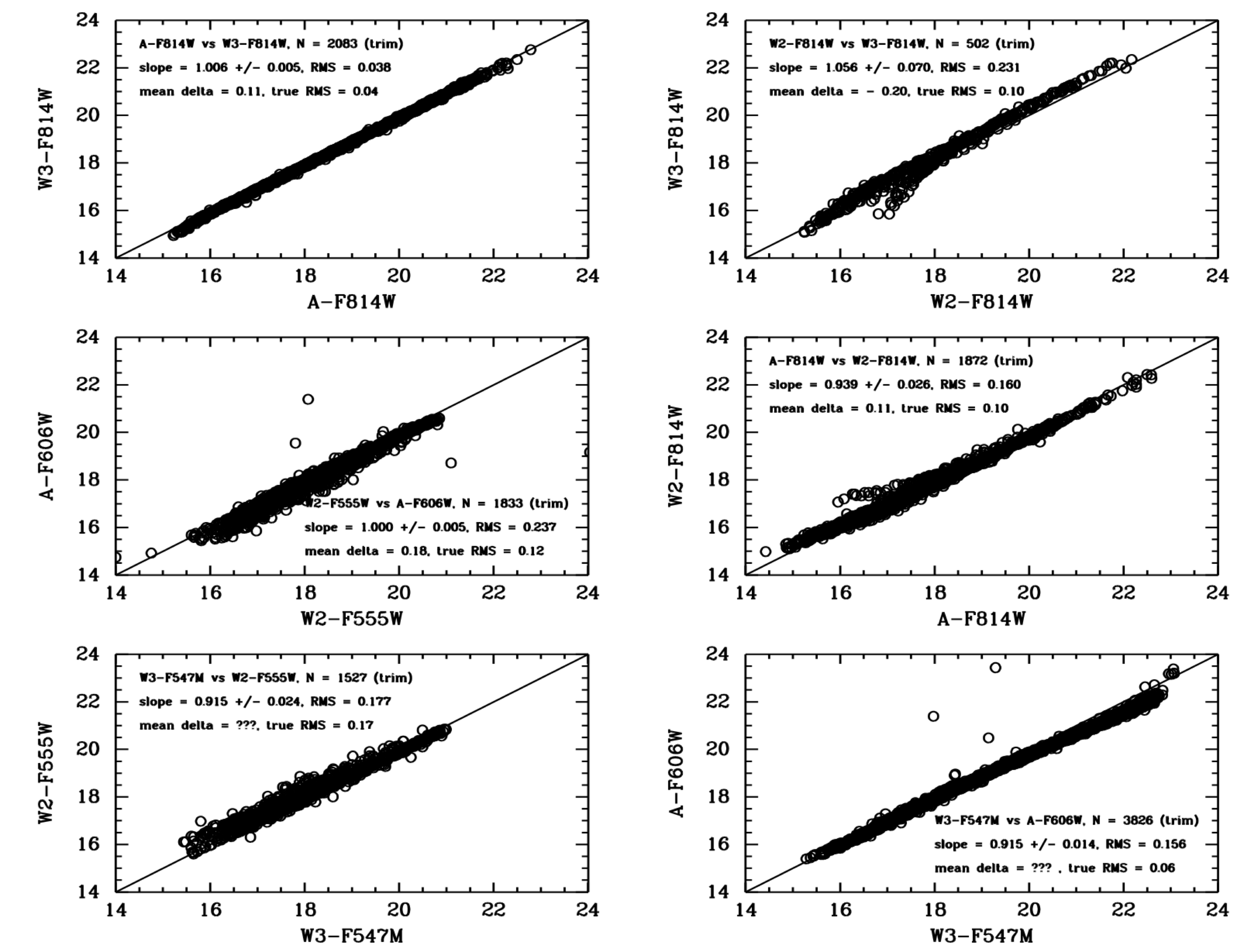
Due to the diversity of the Hubble data, this is a hard question to answer. We have taken a three-pronged approach to address it. We first examine a few specific datasets, comparing magnitudes directly for repeat measurements. The second approach is to compare repeat measurements in the full database. While this provides a better representation of the entire dataset, it can also be misleading since the tails of the distributions are generally caused by a small number of bad images and bad source lists. The third approach is to produce a few well-known astronomical figures (e.g., color-magnitude diagram for the outer disk of M31 from Brown et al 2009) based on HSC data, and compare them with the original study.For our first case we examine the repeat measurements in the globular cluster M4. For this study, as well as the next two, we use MagAper2 values (i.e., aperture magnitudes), which are the default for the HSC. In the last example (extended galaxies) we use MagAuto values.
The figure shows that in general there is a good one-to-one agreement for repeat measurements using different instruments with similar filters. Starting with the best case, A-F814W vs W3-F814W shows excellent results, with a slope near unity, values of RMS around 0.04 magnitudes, and essentially no outliers. However, an examination of the W2-F814W vs. W3-F814W and A-F814W vs W2-F814W comparisons show that there is an issue with a small fraction of the WFPC2 data. The short curved lines deviating from the 1-to-1 relation show evidence of the inclusion of a relatively small number of slightly saturated star measurements (i.e., roughly 5 % of the data).
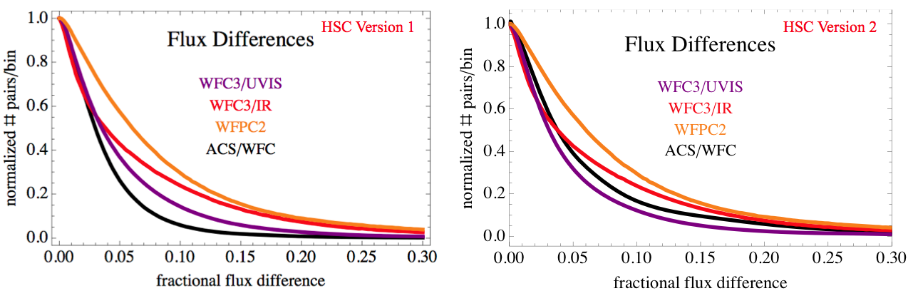
We now turn to our second approach; looking at repeat measurements for the entire HSC database. The following figures shows the distribution of comparisons between independent photometric measurements of pairs of sources that belong to the same match and have the same filter in the HSC for Version 1 and Version 2. The x-axis is the flux difference ratio defined as abs(flux1-flux2)/max(flux1,flux2). The y-axis is the number of sources per bin (whose size is a flux difference ratio of 0.0025) that is normalized to unity at a flux difference of zero.
The main point of this figure is to demonstrate that typical photometric uncertainties in the HSC are better than 0.10 magnitude for a majority of the data. We also note that the curves are quite similar in Versions 1 and 2, with the ACS/WFC becoming somewhat higher at faint magnitudes in Version 2 due to the inclusion of deeper source lists.
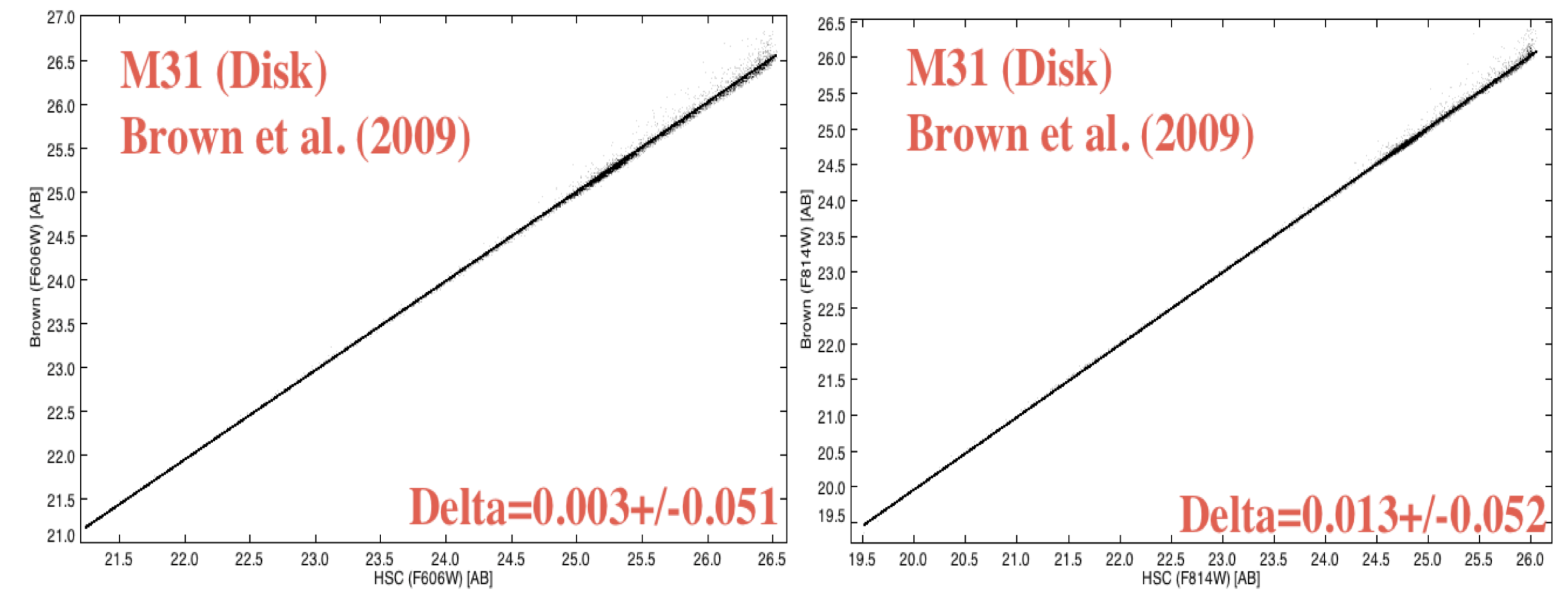
Next we compare HSC data with other studies. The case shown below is a comparison between the HSC and the Brown et al. (2009) deep ACS/WFC observations of the outer disk of M31 (proposal = 10265). The observing plan for this proposal resulted in 60 separate one-orbit visits (not typical of most HST observations), hence provide an excellent opportunity for determining the internal uncertainties by examining repeat measurements. In the range of overlap, the agreement is quite good, with zeropoint differences less than 0.02 magnitudes (after corrections from ABMAG to STMAG and from aperture to total magnitudes) and mean values of the scatter around 0.05 mag. However, the Brown study goes roughly 3 magnitudes deeper, since they work with an image made by combining all 60 visits. More details are available in HSC Use Case #1, and in (Whitmore et al. 2016).
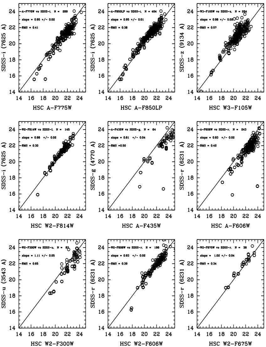
For our final photometric quality example we compare the HSC with ground-based observations from the Sloan Digital Sky Survey (SDSS) observations of galaxies in the Hubble Deep Field. Using MagAuto (extended object photometry) values in this case rather than MagAper2 (aperture magnitudes), we find generally good agreement with SDSS measurements. The scatter is typically a few tenths of a magnitude; the offsets are roughly the same and reflect the differences in photometric systems, since no transformations have been made for these comparisons. The best comparison is between A_F814W and SDSS-i. This reflects the fact that these two photometric systems are very similar, hence the transformation is nearly 1-to-1 .
-
How does the HSC version 2 photometry compare with version 1?
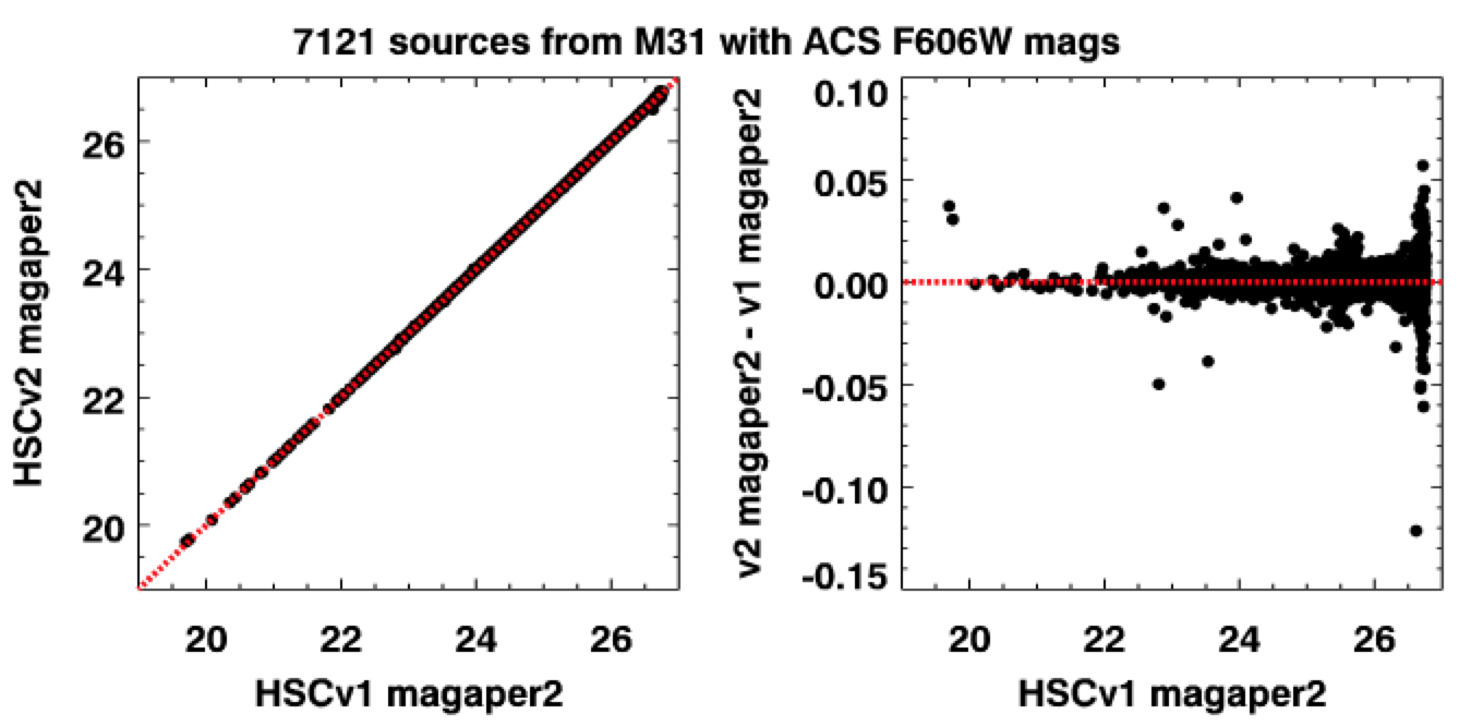 In this figure we compare photometry
from version 2 and version 1 in
a field in M31. This figure was made by requiring
the same individual measurements are present in
both versions, so that we are comparing "apples with apples". We find that the agreement is very
good, with typical uncertainties of a few hundreds of a magnitude.
Similar comparisons (e.g., in M87 where most
of the point-like sources are actually resolved
globular clusters) show similar results.
In this figure we compare photometry
from version 2 and version 1 in
a field in M31. This figure was made by requiring
the same individual measurements are present in
both versions, so that we are comparing "apples with apples". We find that the agreement is very
good, with typical uncertainties of a few hundreds of a magnitude.
Similar comparisons (e.g., in M87 where most
of the point-like sources are actually resolved
globular clusters) show similar results.
If we relax the constraint that the individual measurements be available in both versions we find slightly worse agreement. In particular, we find a tendency for version 2 to have larger values of the RMS sigma values, as included in the summary form. This is primarily due to the inclusion of fainter (noiser) measurements in version 2. However, we find that the mean, and especially the medians, are not greatly affected.
A more detailed description of these comparisons will be included in this section in the future.
-
What is the "Normalized" Concentration Index and how is it calculated??
In version 1, one of the items in the List of "Known Problems" was that raw values of the Concentration Index (the difference in magnitude for aperture photometry using magaper1 and magaper2) were added together to provide a single mean value in the summary form. The reason this is a problem is that each instrument/filter combination has a different normalization. For example, the Peak of Concentration Index for Stars and Aperture Correction Table shows the raw values of the concentration index for stars is 1.08 for the ACS_WFC_F606W filter, 0.88 for WFC3_UVIS_F606W and 0.86 for WFPC2_F606W. Similarly, the raw values of the concentration index vary as a function of wavelength for some detector. For example, WFC3_F110W has a peak value of 0.56 while WFC3_160W has a value of 0.67.
Hence, averaging the mean values of the Concentration Index together in Version 1 resulted in values that were not always very useful, and were often misleading.
In version 2 we have corrected this by normalizing (dividing by) the value of the peak of the raw concentration index for stars using observations from each instrument and filter, as provided in the table listed above. The values are then averaged together to provide an estimate of the "Normalized" Concentration Index, which is listed as the value of CI in version 2 of the summary form.
Hence, objects with values of CI ~ 1.0 are likely to be stars while sources with much larger values of CI are likely to be extended sources, such as galaxies. There are cases where this is still not true (e.g., saturated stars, cosmic rays, misaligned exposures within a visit, ...), hence caution is still required when using values of CI. -
How good is the astrometry for the HSC?
This plot from version 1 shows (in blue) the distribution of the relative astrometric errors in the HSC corrected astrometry, as measured by the positional offsets of the sources contributing to multi-visit matches from their match positions. The units for the x-axis are milli-arcsec (mas). The y-axis is the number of sources per bin that is 0.1 mas in width. Plotted in orange is the corresponding distributions of astrometric errors based on the original HST image astrometry. The peak (mode) of the HSC corrected astrometric error distribution in HSC version 1 was 2.3 mas, while the median offset was 8.0 mas. The original, uncorrected (i.e., current HST) astrometry has corresponding values of 9.3 mas and 68 mas, respectively.
The following two figures show the corrected astrometric offset distributions for the different instruments for multi-visit matches in the HSC for version 1 and version 2. The distribution is actually flatter for version 2, largely due to the inclusion of fainter ACS sources with correspondingly larger pointing uncertainties. Also note the large increase in the number of ACS/WFC sources, due both to the deeper source lists and the addtion of four more years of data!
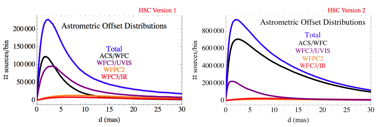
As expected, the instruments with smaller pixels (ACS [50 mas] and WFC3/UVIS [40 mas]) show the best astrometric accuracy, with a peak less than a few mas and typical values less than 10 mas. On the other hand, the instruments with larger pixels WFPC2 [100 mas on the WFC chips which dominate the statistics] and WFC3/IR [130 mas], have much larger astrometric uncertainties, with less than 10 mas peaks and typical values that are less than 20 mas.
Several astrometric studies are currently being analyzed and will be added to this FAQ in the future.
-
How does the HSC compare with Gaia astrometry?
-
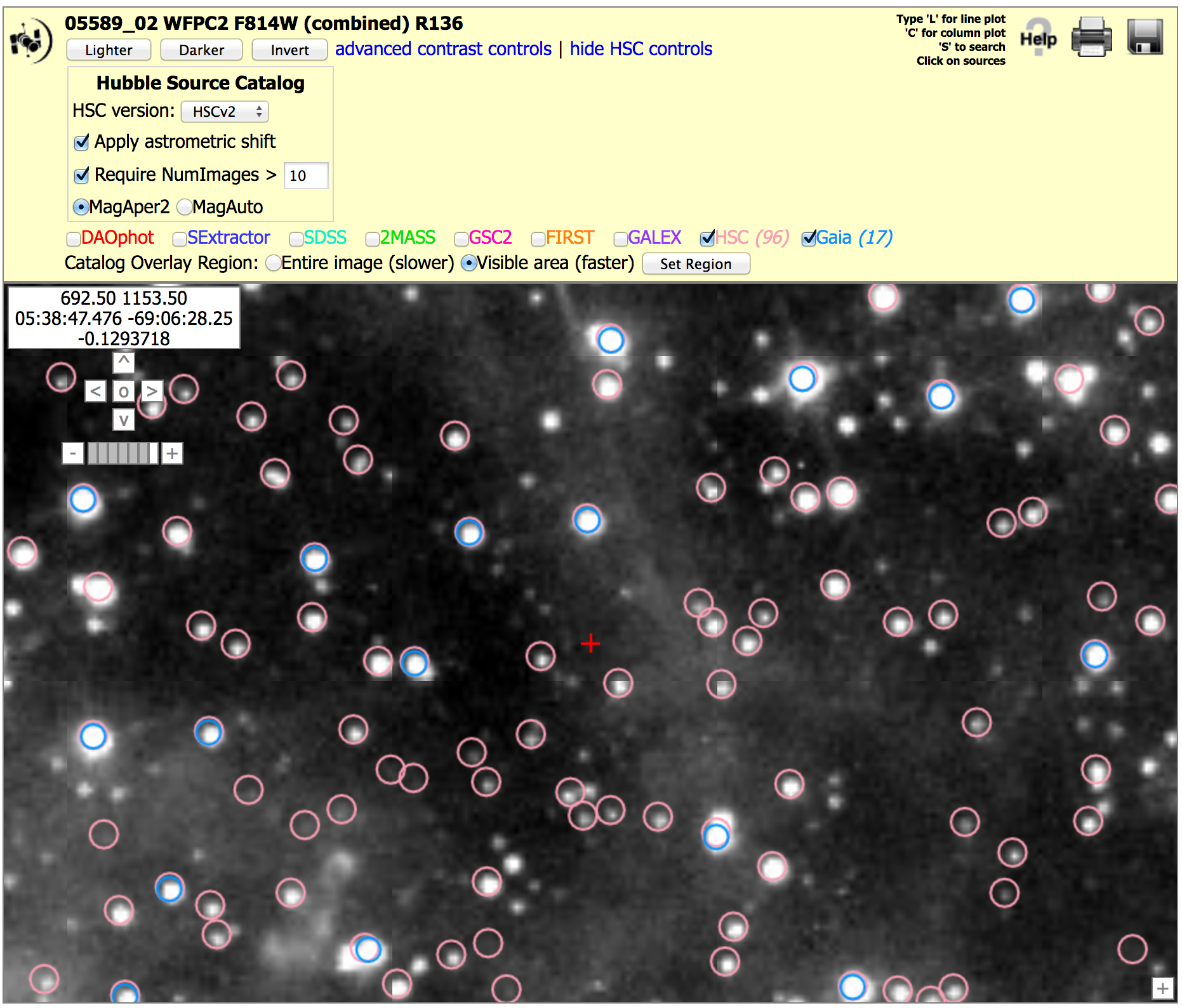
This figure shows a small portion in the outskirts of 30 Dor. There are 17 Gaia sources (blue) in this region and 96 HSC sources (pink) with NumImages > 10. There would be 279 HSC sources if we used a NumImages > 5 criteria to reach fainter sources. This figure shows good agreement in the positions of HSC relative to Gaia for this field. More detailed analysis are currently underway and will be added to this section in the future.
-
What are the future plans for the HSC?
- Improve the WFPC2 sources lists using the newer ACS and WFC3 pipelines.
- Address the known problems in HSC Version 2.
- Integrate the Discovery Portal more fully with the HSC.
- Use mosaic-based (rather than visit-based) source detection lists, and perform forced photometry at these locations on all images.
-
-
Are there training videos available for the HSC?
Yes. There are two videos available:
NOTE: The videos were made using version 1, hence some of the forms and numbers will look somewhat different. However, most of the changes are relatively minor, hence the videos are still useful. New videos will be developed in the future months.
Using the Discovery Portal to search for Variable Objects in the HSC
Using CasJobs with the HSCThere is also a Hubble Hangout that features the HSC.
-
Are there Use Cases available for the HSC?
Yes. We have a variety of Use Cases:
HSC Use Case #1 - Using the Discovery Portal to Query the HSC - (Stellar Photometry in M31 - Brown et al. 2009)
HSC Use Case #2 - Using CASJOBS to Query the HSC - (Globular Clusters in M87 and a Color Magnitude Diagram for the SMC)
HSC Use Case #3 - Using the Discovery Portal to search for Variable Objects in the HSC - (Time Variability in the dwarf irregular galaxy IC 1613)
HSC Use Case #4 - Using the Discovery Portal to perform cross-matching between an input catalog and the HSC - (Search for the Supernova 2005cs progenitor in the galaxy M51)
NOTE: This use case was made using version 1. However, most of the changes are relatively minor, hence it is still quite useful.HSC Use Case #5 - Using the Discovery Portal and CasJobs to search for Outlier Objects in the HSC - (White dwarfs in the Globular Cluster M4)
HSC Use Case #6 - Using the Discovery Portal to study the Red Sequence in a Galaxy Cluster - (The Red Sequence in the Galaxy Cluster Abell 2390)
NOTE: This use case was made using version 1. However, most of the changes are relatively minor, hence it is still quite useful.HSC Use Case #7 - Comparing HSC "Sloan" filter magnitudes and SDSS magnitudes - (using the field around GRB110328A)
NOTE: This use case was made using version 1. However, most of the changes are relatively minor, hence it is still quite useful.HSC Use Case #8 - Combining HSC magnitudes and HST spectra to Investigate Objects in the HSC (using objects in the LMC Cluster R136)
HSC Use Case #9 - Searching for Objects with both HST Imaging and Spectroscopic Data
HSC Use Case #10 - Using the HSC to determine positions for a JWST NIRSpec Multi-Object Spectroscopic (MOS) observation
Archived Use Cases from Beta 0.2
NOTE: These archival use cases are outdated, but included here since they provide some detailed information that may be of interest to people. They do not make use of the Discovery Portal, or CasJobs interface, and they may contain features that are no longer included in the HSC interfaces (e.g., VOPLOT).
-
Is there a facebook page available to share information (e.g., your own use cases) about the HSC ?
 Yes. HSC Facebook Page
Some of the items posted have been:
February 26, 2015 - Comparing HSC and SDSS photometry of galaxies. This was eventually included in the (Whitmore et al. 2016) article.
March 17, 2015 - Announcement of a Hubble Hangout featuring the HSC.
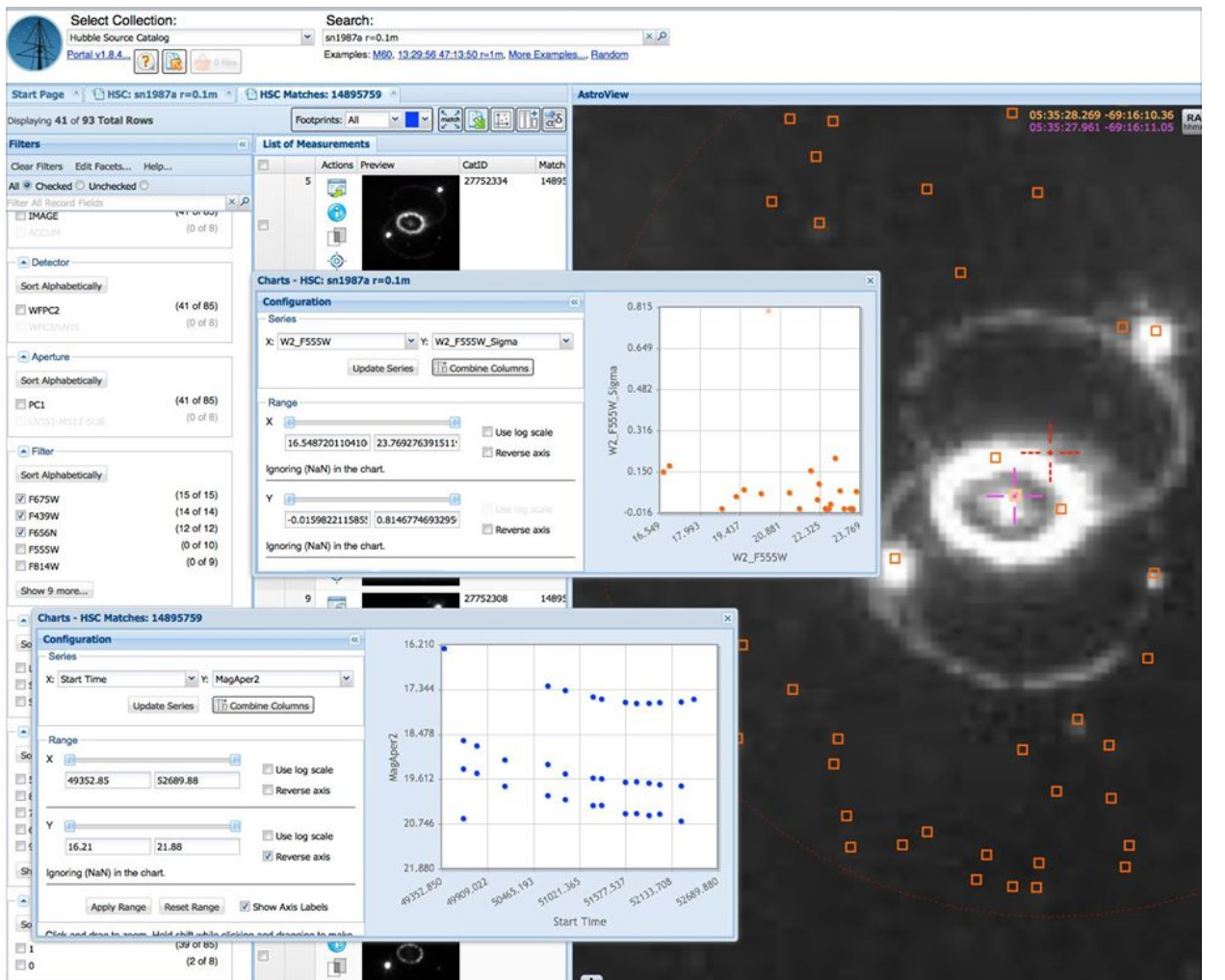
May 6, 2015 - Making a light curve for SN 1987A (see figure).
We plan to include more material following the version 2 release - (e.g., draft use cases, plans for a citizen science project to help characterize HLA images, development of educational modules based on the HLA and HSC, preparations for "Detecting the Unexpected" workshop to be held February 27 - March 2, 2017, potential science projects with the HSC, ...). Please consider joining us so we can develop this into a useful community resource.
-
Is there a journal-level article on the HSC available for reference?
Yes. Whitmore et al. (2016), titled "Version 1 of the Hubble Source Catalog"
There is an updated description of the Beta version of the HSC, and the matching algorithms used in Version 1 in Budavari & Lubow (2012). -
How should I acknowledge that I have used HSC data in my papers?
The HSC is based on data from the Hubble Legacy Archive (HLA). Refereed publications making use of the HSC should therefore include this footnote in the acknowledgements.
"Based on observations made with the NASA/ESA Hubble Space Telescope, and obtained from the Hubble Legacy Archive, which is a collaboration between the Space Telescope Science Institute (STScI/NASA), the Space Telescope European Coordinating Facility (ST-ECF/ESAC/ESA) and the Canadian Astronomy Data Centre (CADC/NRC/CSA)."
Authors are also asked to acknowledge the "Hubble Source Catalog" in the text of the paper, and reference the Whitmore et al. (2016) paper, if appropriate. -
Send a note to archive@stsci.edu. Please include enough information (e.g., a screen save of the problem) to make it possible to diagnose any problems.
FAQ - About Spectroscopic Cross Matching
For HSC version 2.1, spectroscopic matches for COS, FOS, and GHRS observations have been added for Version 2 sources that do not have Version 1 counterparts. In general you will find the same matches in Version 2.1 as Version 2, but you will also find additional new matches for a small number of objects. An example can be seen by searching for MRK817 using the Discovery Portal (i.e., match ID = 12904924). This was not a spectroscopic match for Version 2 but now is for Version 2.1 .
Another resource that may be of interest is the HST Spectroscopic Legacy Archive (HSLA). At present, this only provides access to COS FUV data. The HSC spectroscopic cross matching and the HSLA will be more closely linked in the future. Another resource that may be of interest is the HST Spectroscopic Legacy Archive (HSLA). At present, this only provides access to COS FUV data. The HSC spectroscopic cross matching and the HSLA will be more closely linked in the future.
For the other spectrographs, manual matching of the spectral object with the HSC was performed. First, an automated matching was performed with a search radius of 3.0 arcsec. If no HSC object was detected for a spectrum it was assumed there was no corresponding HSC source. Note that this does not mean that there might not be an image, or a source not included in the HSC, as discussed in the "Current Limitations" section of the Hubble Source Catalog home page.
If there was an HSC object, then the imaging data was inspected visually to identify the object. The identification was based on both the coordinate match as well as a rough magnitude match. For the FOS and GHRS, the targets were all bright enough that there was typically only one valid match candidate. For crowded fields, and for COS which observed fainter targets, finding charts from the literature were used (when possible) to confirm the identifications.
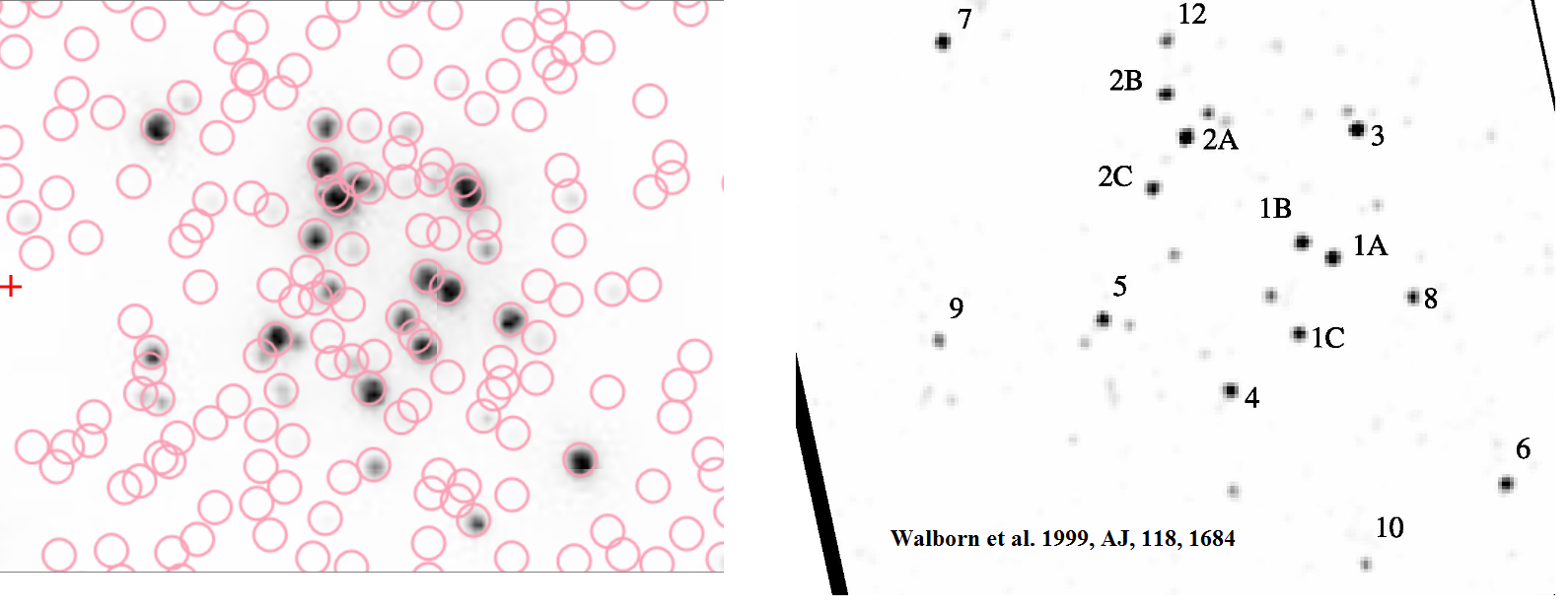 For example, this figure shows how
(Walborn et al. 1999)
was used to identify matches in 30 Dor.
For example, this figure shows how
(Walborn et al. 1999)
was used to identify matches in 30 Dor.
For some cases, either the finding chart was not sufficient, or there were no charts available, so no definite match could be made. These spectra are included in the spectral database with the HSC Match value being set to No. They are included to make users aware there is imaging data available, and that if a finding chart could be found it may be possible to match the spectrum with an HSC object.
For extended sources, it was sometimes not possible to determine exactly where the spectrum was obtained. If there was a clear knot/bright spot at the coordinates of the spectra, and that spot was identified as an HSC object, then a match was considered likely. However, all matches in extended objects should be considered as likely matches only.
Similarly, the object type included with the spectral data was generally obtained from the original proposer's classification in the Target Description field. However, in some cases, the same target was observed by multiple proposers, and the object types were different in the proposals. For these cases, other sources (e.g. Simbad, literature) were used to select a single type.
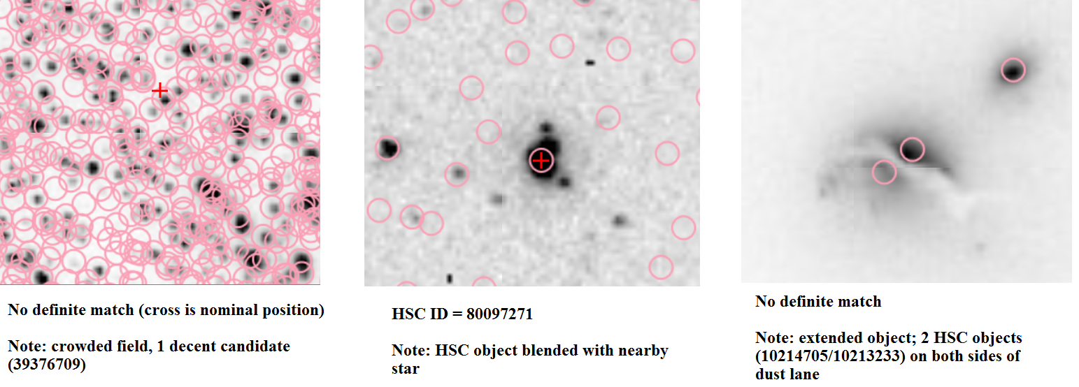 When doing the manual matching, sometimes there were issues with
the imaging data (e.g. crowded field, extended object) that
could impact the quality of the match between the HSC and the spectral data.
This information is included in the notes, as shown in these three examples.
When doing the manual matching, sometimes there were issues with
the imaging data (e.g. crowded field, extended object) that
could impact the quality of the match between the HSC and the spectral data.
This information is included in the notes, as shown in these three examples.
See HSC Use Case # 8 and 9 for more examples.
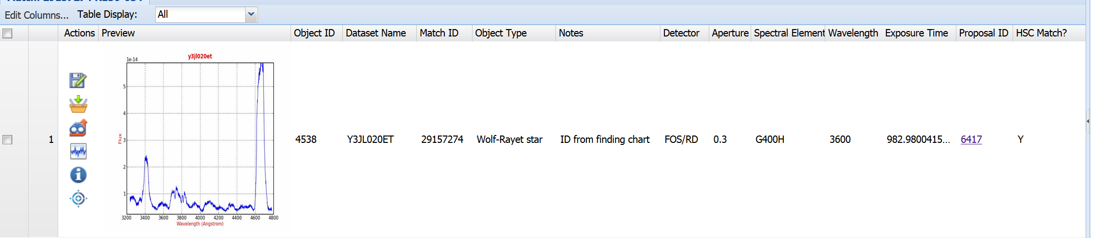 Here is an example of a match used in Use Case #8 (i.e., HSC MatchID=29157274)
The following columns are found in the spectral results page:
a) Preview - a preview image of the spectrum
b) Object ID - the ID number in the spectrum database
c) Dataset Name - the name of the dataset in the Archive
d) Match ID - the HSC Match ID number. See details about how the matching was done.
e) Object Type - the classification of the object. See details about how the classification was done.
f) Notes - when applicable, notes about the matching of the spectral observation with the HSC data (e.g. for crowded fields, the ID is based on a published finding chart and not just a coordinate match)
g) Detector, Aperture, Spectral Element, Wavelength, Exposure Time - the exposure parameters for the spectrum from the Archive
h) Proposal ID - the ID number of the proposal that generated the spectrum. Clicking on this will show you the abstract.
i) HSC Match? - if Yes, then there is an HSC match for the spectral. If No, then there was imaging data available, but no HSC match was identified (either because there was no object at the coordinates of the object or there were multiple candidates)
 icon in the MAST Discovery Portal you will
get the HSC photometric summary page for the object. See HSC Use Case # 8 for an example.
icon in the MAST Discovery Portal you will
get the HSC photometric summary page for the object. See HSC Use Case # 8 for an example.
FAQ - About Accessing the HSC
-- Searching and filtering the HSC database.
-- Viewing the HSC or filtered subsets overplotted on images (e.g, DSS, GALAX, SDSS, and HST). Access to the HLA Interactive Display is also available.
-- Viewing the HSC in a table format. Creating new columns and plotting one column vs. another.
-- Cross matching with a wide range of surveys including GALEX, SDSS, 2MASS, as well as tables available from CDS (Strasbourg Astronomical Database).
-- Uploading or downloading tables data from/to local files.
-- And as of HSC version 2, showing spectroscopic data from the ACS Grisms, COS, FOS and GHRS cross matched with the HSC. See the FAQ - About Spectroscopic Cross Matching for details.