 |
This chapter describes the science data files available from the FUSE
archive. Ancillary data files, which provide additional information about the
state of the instrument and spacecraft, are described in Chapter 5.
The "Casual" user mostly needs to examine FUSE preview files and understand their limitations while the "Intermediate" and "Advanced" users need to be knowledgeable about some or all of the FUSE data files for an observation. Table 4.1 in the next section lists all FUSE data file extensions available for download from the MAST archive. This table is aimed at helping all users determine which files are essential to their project and to find the relevant information throughout this document. It is, therefore, strongly recommended that potential FUSE users read the Overview Section (below) and familiarize themselves with the contents of these tables before retrieving any data files.
A FUSE observation is a set of contiguous exposures of a
particular target through a specific aperture. Each exposure generated
four raw science data files, one for each detector segment (1A, 1B, 2A and
2B). There are two pairs of spectra (one LiF and one SiC) for the target on
each detector segment. When all of the data are extracted, 8 calibrated
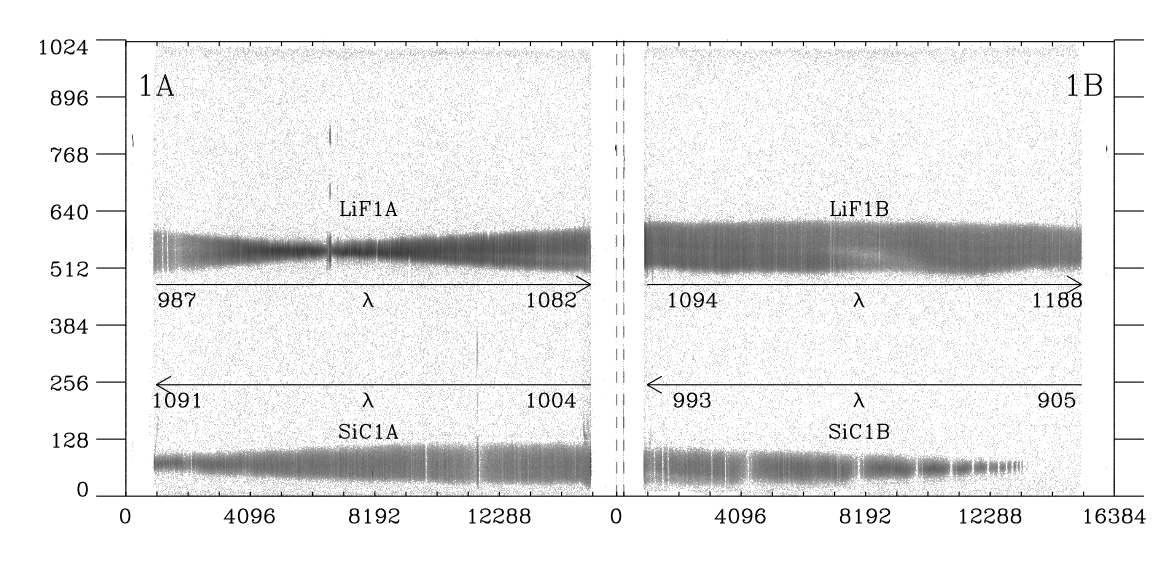
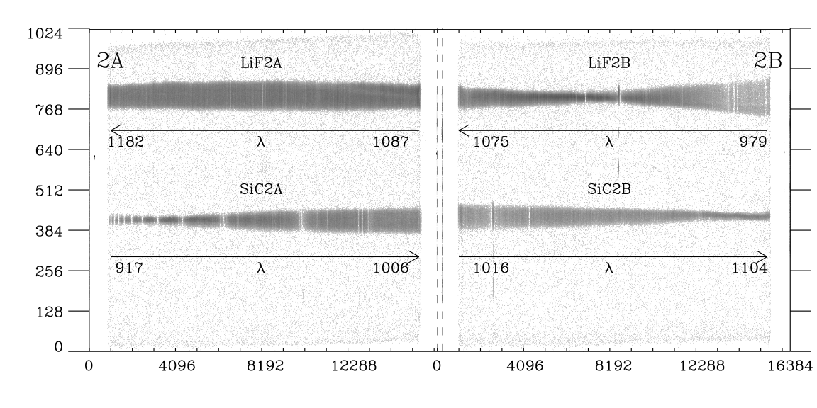
spectra result from a single exposure. Figures 4.1
and 4.2 show
geometrically corrected images of spectra on Side 1 and Side 2 detectors for a single
exposure. Observations may consist of any number of exposures between 1 and
(in principle) 999.
Spectra are extracted by CalFUSE only for the target aperture and are binned in
wavelength. The default binning is 0.013 Å, which corresponds to about
two detector pixels, or one fourth of a point source resolution element.
After processing, a series of combined observation-level
spectral files are generated along with a variety of preview files.
These files will be discussed in detail in the next sections.
FUSE spectra are susceptible to a variety of systematic effects that are
described in detail in Chapter 7. These systematics can
affect a portion or all of a spectrum from one or more channel and detector
combinations. Hence, it is important to compare channels with overlapping
wavelength ranges for consistency (see Table 2.2). A discrepancy between the
spectra from overlapping channels may indicate the presence of one or more of
these effects. Such systematic errors may be considerably larger
than the statistical errors provided in the extracted spectra.
|
 |
All FUSE data are stored as FITS files containing one or more Header +
Data Units (HDUs). The first is called the primary HDU (or HDU1); it
consists of a header and an optional N-dimensional image array. The
primary HDU may be followed by any number of additional HDUs, called
"extensions". Each extension has its own header and data unit. FUSE
employs two types of extensions, image extensions (2-dimensional array) and
binary table extensions (rows and columns of data in binary
representation). FITS files can be read by a number of general and
astronomical software packages (see Chapter 8).
Table 4.1 lists all the files types available for retrieval from the MAST archive interface. In the table the following are listed: Column (1), file types; Column (2), detector side; Column (3), detector segment; Column (4), channels; Column (5), aperture used for observation; Column (6), observing mode; Column (7), data type; Column (8), section where each file is discussed; and Column (9), "Expertise Level" corresponding to the readers' motivation for using FUSE data: Casual (Cas), Intermediate (Int), or Advanced (Adv; see Chapter 1). Hence, inspection of this table will provide the user with instant information about 1) which files are required for his/her purposes, and 2) in which sections those files are discussed in detail throughout this document.
| File Types | Side | Segment | Channel | Aperture | Mode | Type | Section | Expertise |
|---|---|---|---|---|---|---|---|---|
| Raw Files | ||||||||
| fraw.fit | 1, 2 | a, b | … | … | ttag, hist | photon list, image | 4.2.1.1 | Adv |
| fes*raw.fit | a, b | … | … | … | … | raw FES | 5.1 | Adv |
| snapf.fit | … | … | … | … | … | engineering snapshot file | 5.3 | Adv |
| snp*f.fit | a, b | … | … | … | … | FES associated snapshot | 5.3 | Adv |
| hskpf.fit | … | … | … | … | … | housekeeping table | 5.2 | Adv |
| jitrf.fit | … | … | … | … | … | jitter table | 5.2 | Adv |
| Calibrated Files | ||||||||
| *fcal.fit | 1, 2 | a, b | SiC, LiF | 2, 3, 4 | ttag, hist | spectrum | 4.2.1.2 | Int, Adv |
| *00all*fcal.fit | … | … | … | 2, 3, 4 | ttag, hist | header | 4.2.2.1 | Int, Adv |
| *00000all*fcal.fit | … | … | … | 2, 3, 4 | ttag, hist | spectrum | 4.2.2.1 | Cas, Int, Adv |
| *00000ano*fcal.fit | … | … | … | 2, 3, 4 | ttag, hist | spectrum | 4.2.2.1 | Int, Adv |
| *fidf.fit | 1, 2 | a, b | … | … | ttag, hist | photon list (IDF) | 4.2.1.3 | Adv |
| *f.trl | 1, 2 | a, b | … | … | ttag, hist | processing trailer | 4.2.1.5 | Int, Adv |
| *asnf.fit | … | … | … | … | … | association table | 5.4 | Int, Adv |
| *fes*fcal.fit | a, b | … | … | … | … | calibrated FES image | 5.1 | Adv |
| *hskpf.fit | … | … | … | … | … | housekeeping table | 5.2 | Adv |
| *jitrf.fit | … | … | … | … | … | jitter table | 5.2 | Adv |
| Preview Files | ||||||||
| *fext.gif | 1, 2 | a, b | … | … | ttag, hist | extraction window plot | 4.2.1.4 | Int, Adv |
| *frat.gif | 1, 2 | a, b | … | … | ttag, hist | count-rate plot | 4.2.1.4 | Int, Adv |
| *00000*f.gif | 1, 2 | … | SiC, LiF | … | ttag, hist | plot | 4.2.2.2 | Cas, Int, Adv |
| *00000*spec*f.gif | … | … | … | … | ttag, hist | plot | 4.2.2.2 | Cas, Int, Adv |
| *00000*nvo*fcal.fit | … | … | … | … | ttag, hist | spectrum | 4.2.2.2 | Cas, Int, Adv |
All FUSE file names are composed of several identifying elements, but not all files contain each one of these elements. However, all exposure-level file names have the form {pppp}{tt}{oo}{eee} and begin with the following four elements:
FUSE program ID codes convey general information about the category of the program, be it primarily for science or calibration. As indicated in Tables 4.2, 4.3 and 4.4, the dividing line is not hard. Sometimes useful science data can be extracted from data that were obtained for calibration purposes (for example, the flux calibration programs). Other times, the requirements of the calibration activity itself may seriously compromise the use of any spectral data for science. For some `I' programs (in-orbit checkout), the data may be useful for science but only with great caution since the instrument may not have reached its final science configuration and focus yet. Many targets observed during in-orbit checkout were re-observed later in the mission, and the user should be wary of the IOC observation. However, these data are archived at MAST, so the user should be cognizant. Information on the sequence of instrument focus activities during in-orbit checkout can be found in the Instrument Handbook (2009); this may assist the user in evaluating the utility of the IOC observations.
| Code | Category |
|---|---|
| Annn | Cycle 1 Guest Investigator (GI) programs |
| Bnnn | Cycle 2 GI programs |
| … | … |
| Hnnn | Cycle 8 GI programs |
| Pnnn | PI Science team guaranteed time (US) |
| Qnnn | PI Science team guaranteed time (France) |
| Sn05 | [n=4-9] Sky Background Observations |
| Unnn | Non-proprietary re-observations of science targets |
| Xnnn | Early Release Observations (EROs) |
| Z0nn | Project Scientist Discretionary Programs |
| Z9nn | Observatory Programsa |
| a Observatory programs were non-peer-reviewed science programs executed at the discretion of the NASA Project Scientist. These programs were designed to fill a gap in science target availability after the initial reaction wheel problems in late 2001. | |
| Code | Category |
|---|---|
| I8nn | Spectrograph Focus and Alignment |
| I904 | Random Science fillers |
| M10nb | Calibration/Maintenance Programs |
| S601-701 | Science Verification (SV) programs |
| a These data might reveal interesting science. For example, McCandliss (2003) used wavelength-calibration data from program
M107.
b See Table 4.4 for exceptions. | |
| Code | Category |
|---|---|
| Innnb | Instrument In-Orbit Check-out (IOC) programs |
| Mn12-n14 | Periodic Alignment Programs, [n=1,2] |
| M717-727 | Channel Alignment |
| M9nnb | Detector Characterization Programs |
| Snnnb | Science Verification (SV) programs |
| a These data should NOT be used for science purposes because they were typically obtained with settings far from nominal. The spectra, if they exist for these programs, suffer from unusual systematic effects. | |
NOTE 1: Two types of airglow observations were obtained during the course of the mission: i) dedicated bright-earth observations (see Chapter 9); and ii) airglow exposures obtained as part of a science program execution. Observations (i) are archived under program codes M106 and S100. Airglow exposures (ii) are archived with their respective science program codes. They are assigned exposure numbers >900 to distinguish them from the regular science exposures. For further details, see the NOTES in Sections 4.2.1.2, 4.2.1.3, and 4.2.2.1. A separate interface to retrieve airglow data is available at the MAST archive.
NOTE 2: Separate from airglow observations are sky background observations, found in programs S405, S505, S605, S705, S805, and S905. The FUSE sky backgrounds program started in an attempt to get potentially scientifically useful data during thermalization periods prior to channel alignment activities (when normal science observing could not be done). For programs S405 and S505 targets, the alignment target was placed at the RFPT and thus the "sky" position was a randomly-accessed region roughly an arcminute away (exact position dependent on the roll angle, hence the day of observation). Multiple observations of the same target in these programs thus do not correspond exactly to the same piece of sky, but for diffuse emission it was not expected to matter very much.
Beginning in 2005, after the reaction wheel problems, it became useful to define sky positions in stable regions of the sky, to provide targets for stable pointing when no regular science target was available. Again, the intent was to obtain science data from periods that would otherwise have gone to no good purpose. These include programs S605, S705, S805, and S905. These were all pointed observations, so the given coordinates correspond to the LWRS aperture for these observations. Hence, multiple observations in these programs correspond to the same piece of sky, albeit with a different aperture position angle (which should be negligible).
It is gratifying that these observations have resulted in interesting diffuse background measurements. The reader is referred to Dixon et al. (2006) and references therein.
The alignment scan observations involved stepping a star across the LWRS aperture in each channel. Correlation of photon events with pointing position and reconstruction of a spectrum may be possible. However, in most instances the effective exposure time will be short and the results will not warrant the labor involved.
Because up to eight spectral files can be produced by a single FUSE exposure, and since a single observation can be composed of multiple exposures, we introduce a compressed notation to summarize the different sets of files. In the following, we depict file names as a group of italic and typewriter type faces, as indicated in Table 4.5.
| Typeface | Group property |
|---|---|
| italic | variable which depends on a specific file |
| typewriter | always present |
| typewriter array | each combination is always present. |
Two variables that often appear in the file names are the aperture number an = {2,3,4} (see Table 2.1), and the data collection mode = {ttag, hist} (see Section 2.1.7). A target can also be placed at the reference point (RFPT). In that case, data from the LWRS aperture are extracted and archived by CalFUSE by default, and the files are labeled with the LWRS code, an = 4.
NOTE: The string "cal" appearing in FITS file names stands for "calibrated" and indicates that the data have been completely processed through CalFUSE; see (Dixon et al. (2007)).
This section describes the names and contents of the FUSE data files. Details of the FITS header keywords are given in Chapter 6.
CalFUSE creates several data (FITS) and preview (GIF) files for each
exposure. We begin with the unprocessed raw data files (*fraw.fit) and continue through
the various levels of processing. In this case, there are two levels of processing:
the extracted spectral files (*fcal.fit) and the intermediate data files (*fidf.fit).
RAW data files contain the unprocessed science data. There is one RAW file for each detector
segment. The RAW file names have the following format:
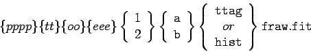
The contents of the RAW TTAG and HIST data files are different. RAW TTAG data are saved as event lists. In the TTAG FITS file, HDU1 is empty, containing only a header, HDU2 contains a list of time, X, Y and pulse height amplitude (PHA) for all of the photon events, and HDU3 contains the start and stop times of the Good Time Intervals (GTIs). The time resolution is ordinarily 1 second, but in a few instances the resolution was set to 8ms for diagnostic purposes. Note that in the latter case, the IDS-inserted timestamps don't provide an exact representation of 8ms: the effective LSB is closer to 1/128 second instead of 1/125 second. The result is an apparent periodic irregularity in the count rate. For TTAG, the initial GTI values are copied over from raw data files. By convention, the start value of each GTI corresponds to the arrival time of the first photon in that interval. The stop value is the arrival time of the last photon in that interval plus one second. The length of the GTI is thus STOP — START. For HIST data, a single GTI is generated with start = 0 and stop = the exposure time. These are summarized in Table 4.6.
| FITS Extension | Format | Description |
|---|---|---|
| HDU 1: Empty (Header only) | ||
| HDU 2: Photon Event List (binary extension) | ||
| TIME | FLOAT | Photon arrival time (seconds) |
| X | SHORT | Raw X position (0—16383) |
| Y | SHORT | Raw Y position (0—1023) |
| PHA | BYTE | Pulse height (0—31) |
| HDU 3: Good-Time Intervals (binary extension) | ||
| START | DOUBLE | GTI start time (seconds) |
| STOP | DOUBLE | GTI stop time (seconds) |
| a Times are relative to the exposure start time, stored in the header keyword EXPSTART. | ||
RAW HIST observations are transmitted from the satellite as images of the portions of the detector selected in the SIA table. Typically, there are two binned images corresponding to the parts of the detector where the and unbinned in X (with the exception of observations M999 which are binned 2 × 2 and cover the full detector) and, depending upon the channel, the images are usually 16384 in X, and between 12-20 binned pixels in Y. In addition to these data, the RAW HIST file also contain two 2048 × 2 images of the regions containing the stim pulses. These are used to determine the amount of drift in the image (see Chapter 2). Table 4.7 summarizes the contents of the RAW HIST data files.
| FITS Extension | Description | Format |
|---|---|---|
| HDU | Contents | Image Sizea (binned pixels) |
| 1b | SIA Tablec | 8 × 64 — BYTE |
| 2 | SiC Spectral Image | 16384 × (12—20) — INT |
| 3 | LiF Spectral Image | 16384 × (12—20) — INT |
| 4 | Left Stim Pulse | 2048 × 2 — INT |
| 5 | Right Stim Pulse | 2048 × 2 — INT |
|
a Quoted image sizes assume the standard histogram binning: unbinned in X, by 8 pixels in Y. Actual binning factors are given in the primary file header and keywords SPECBINX, SPECBINY.
b Header keywords of HDU 1 contain exposure-specific information. c The SIA table indicates which regions of the detector are included in the file (see Section 2.5.2). | ||
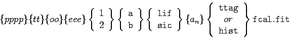
These data are fully calibrated, extracted spectra for each channel and
segment. The spectra are extracted only for the science aperture and specified in
the keyword APERTURE (see Chapter 6). Note that for TTAG data the other
apertures may contain useful information, but one must use the IDF files
(see below) to extract them. For HIST data, spectra are only available for the
science aperture
specified by the observer since the data from the other apertures were not recorded.
Exposure times for TTAG observations can be anything up to the duration of one orbit
for objects observed in the Continuous Viewing Zone (CVZ) because
spacecraft motions and other time-dependent effects can be corrected
in the TTAG photon event list. On the other hand, HIST observations are typically quite short
(about 400 s) in order to minimize Doppler smearing by the motion of the spacecraft.
For a single exposure, CalFUSE produces 8 extracted spectra, named as
follows:
| {FITS Extension} | Format | Description |
|---|---|---|
| HDU 1: Empty (Header only)} | ||
| HDU 2: Extracted Spectrum (binary extension) | ||
| WAVE | FLOAT | Wavelength (Å) |
| FLUX | FLOAT | Flux (erg cm-2 s-1 Å-1) |
| ERROR | FLOAT | Gaussian error (erg cm-2 s-1 Å-1)) |
| COUNTS | INT | Raw counts in extraction window |
| WEIGHTS | FLOAT | Raw counts corrected for dead time |
| BKGD | FLOAT | Estimated background in extraction window (counts) |
| QUALITY | SHORT | Percentage of window used for extraction (0 — 100) |
NOTE: Occasionally, exposures containing airglow emission alone were obtained while executing a science program. To differentiate these data from the science data, the airglow observations were assigned exposure numbers eee > 900 in the spectral file names. The SRC_TYPE keyword is set to EE, and the following warning is written to the file header: "Airglow exposure. Not an astrophysical target."
As processing proceeds, CalFUSE keeps the TTAG data in the form of a photon event list
until spectral extraction. HIST data are converted into a pseudo
event list in which all photons are tagged with the same time value for a given exposure. These event lists
are stored in IDF files. The IDF file is a FITS file with four HDUs comprised of a header and
three FITS binary table extensions
(see Table 4.9). A brief description of each HDUs' content is given below.
For more details, the user is referred to Appendix B of this
document and Dixon et al. (2007).
The first header data unit (HDU1) consists of the header originally copied from the raw data
file. This header is modified as the IDF goes through the different pipeline steps.
This header contains basic information about the proposal, the exposure, the observation,
and the calibration as well as engineering and housekeeping data.
HDU2 is a time-tagged list of photon events with their raw X, Y, coordinates,
weights, and pulse height. Other parameters are set to dummy values at the creation of the
IDF file and later modified as the IDF file runs through the pipeline modules.
HDU3 is the list of good time intervals (see Chapter 5).
Since the events listed in the IDF files are flagged as "good" or "bad" but never
discarded, users can change the event selection criteria without re-running the pipeline.
For example, IDF files can be combined to create a higher S/N image
for more robust spectral extraction of very faint targets. They can be used to
examine the flux and extract spectra in apertures other than the target aperture, or they can
be divided into temporal segments to examine the time-dependence of an object. Brief descriptions
of how to perform such tasks can be found on the MAST webpage in the document
"FUSE Tools in C".
| FITS Extension | Format | Description |
|---|---|---|
| HDU 1: HIST files | BYTE | SIA Table |
| HDU 1: TTAG files | Empty | Header only |
| HDU 2: Photon-Event List (binary extension)} | ||
| TIME | FLOAT | Photon arrival time (seconds) |
| XRAW | SHORT | Raw X position (0—16383) |
| YRAW | SHORT | Raw Y position (0—1023) |
| PHA | BYTE | Pulse height (0—31) |
| WEIGHT | FLOAT | Photons per binned pixel for HIST data; initially 1.0 for TTAG data |
| XFARF | FLOAT | X coordinate in geometrically-corrected frame |
| YFARF | FLOAT | Y coordinate in geometrically-corrected frame |
| X | FLOAT | X coordinate after motion corrections |
| Y | FLOAT | Y coordinate after motion corrections |
| CHANNEL | BYTE | Aperture+channel ID for the photon (Table 4.10) |
| TIMEFLGS | BYTE | Time flags (Table 4.11) |
| LOC_FLGS | BYTE | Location flags (Table 4.12) |
| LAMBDA | FLOAT | Wavelength of photon (Å) |
| ERGCM2 | FLOAT | Energy density of photon (erg cm-2) |
| HDU 3: Good-Time Intervals (binary extension) | ||
| START | DOUBLE | GTI start time (seconds) |
| STOP | DOUBLE | GTI stop time (seconds) |
| HDU 4: Time-Line Table (binary extension) | ||
| TIME | FLOAT | Seconds from exposure start time |
| STATUS_FLAGS | BYTE | Status flags |
| TIME_SUNRISE | SHORT | Seconds since sunrise |
| TIME_SUNSET | SHORT | Seconds since sunset |
| LIMB_ANGLE | FLOAT | Limb angle (degrees) |
| LONGITUDE | FLOAT | Spacecraft longitude (degrees) |
| LATITUDE | FLOAT | Spacecraft latitude (degrees) |
| ORBITAL_VEL | FLOAT | Component of spacecraft velocity in direction of target (km/s) |
| HIGH_VOLTAGE | SHORT | Detector high voltage (digital units) |
| LIF_CNT_RATE | SHORT | LiF count rate (counts/s) |
| SIC_CNT_RATE | SHORT | SiC count rate (counts/s) |
| FEC_CNT_RATE | FLOAT | FEC count rate (counts/s) |
| AIC_CNT_RATE | FLOAT | AIC count rate (counts/s) |
| BKGD_CNT_RATE | SHORT | Background count rate (counts/s) |
| YCENT_LIF | FLOAT | Y centroid of LiF target spectrum (pixels) |
| YCENT_SIC | FLOAT | Y centroid of SiC target spectrum (pixels) |
| a Times are relative to the exposure start time, stored in the header keyword EXPSTART. To conserve memory, floating-point values are stored as shorts (using the FITS TZERO and TSCALE keywords) except for TIME, WEIGHT, LAMBDA and ERGCM2, which remain floats. | ||
Occasionally, photon arrival times in raw TTAG data files are corrupted. When this happens, some fraction of the photon events have identical, usually large TIME values, and the good-time intervals (GTI) contain an entry with START and STOP set to the same large value. The longest valid exposure spans 55 ks. If an entry in the GTI table exceeds this value, the corresponding entry in the timeline table is flagged as bad using the "photon arrival time unknown" flag; (see Dixon et al. (2007)). Bad TIME values less than 55 ks will not be detected by the pipeline.
Raw HIST files may also be corrupted. OPUS fills missing pixels in a HIST image with the value 21865. The pipeline sets the WEIGHT of such pixels to zero and flags them as bad. This is done by setting the photon's "fill-data bit" (see Dixon et al. (2007)). Bad TIME values less than 55 ks will not be detected by the pipeline.
Raw HIST files may also be corrupted. OPUS fills missing pixels in a HIST image with the value 21865. The pipeline sets the WEIGHT of such pixels to zero and flags them as bad. This is done by setting the photon "fill-data bit" (see Dixon et al. [2007]). Single bit-flips are corrected on-board, but occasionally a cosmic ray will flip two adjacent bits. Such double bit- flips are not detected by the correction circuitry, producing (for high-order bits) a "hot pixel" in the image. The pipeline searches for pixels with values greater than 8 times the average of their neighbors, and masks out the higher-order bits.
One or more image extensions may be missing from a raw HIST file. If no extensions
are present, the keyword EXP STAT in the IDF header is set to -1. Exposures with non-zero
values of EXP STAT are processed normally by the pipeline, but are not included in the
observation-level spectral files ultimately delivered to MAST. Though the file contains no data,
the header keyword EXPTIME is not set to zero.
When creating the IDF files for bright-earth observations (programs M106 and S100) or 900-level airglow exposures, CalFUSE sets the header keyword EXP_STAT = 2. For 900-level exposures, the SRC_TYPE is set to EE, and the following warning is written to the file header: "Airglow exposure. Not an astrophysical target." The pipeline then processes the file as usual. In particular, the limb-angle flag is set in the timeline table (extension 3 of the IDF), and the "Time with low limb angle" is written to the file header. However, the following things change:
The extracted spectra include photons obtained at low limb angles. The detector-image plots (*spec.gif) do, too. But the count-rate plots (*ext.gif; *rat.gif) still indicate times when the line of sight passed below the nominal limb-angle limit.
| Aperture | LiF | SiC |
|---|---|---|
| HIRS | 1 | 5 |
| MDRS | 2 | 6 |
| LWRS | 3 | 7 |
| Not in an aperture 0 | ||
| Bit | Value |
|---|---|
| 8 | User-defined bad-time interval |
| 7 | Jitter (target out of aperture) |
| 6 | Not in an OPUS-defined GTI or photon arrival time unknown |
| 5 | Burst |
| 4 | High voltage reduced |
| 3 | SAA |
| 2 | Limb angle |
| 1 | Day/Night flag (N = 0, D = 1) |
| a Flags are listed in order from most- to least-significant bit. | |
| Bit | Value |
|---|---|
| 8 | Not used |
| 7 | Fill data (histogram mode only) |
| 6 | Photon in bad-pixel region |
| 5 | Photon pulse height out of range |
| 4 | Right stim pulse |
| 3 | Left stim pulse |
| 2 | Airglow feature |
| 1 | Not in detector active area |
| a Flags are listed in order from most- to least-significant bit. | |
Two types of exposure-level diagnostic preview files are available, and both serve as
useful tools to verify the integrity of spectra derived from the
exposure.
*rat.gif: These files display the count rate throughout the exposure (see Fig 4.3). For TTAG data, this is the actual count rate for events occurring within the region of the detector corresponding to the target aperture (excluding airglow features) evaluated every second. For HIST data, these are the dead time corrected counter data from the time engineering files (housekeeping file, see Section 5.2), which are sampled once every 16 seconds (see Table 4.9). For non-variable objects, these are useful diagnostics, since they enable the user to determine whether the target remained within the aperture throughout the exposure.
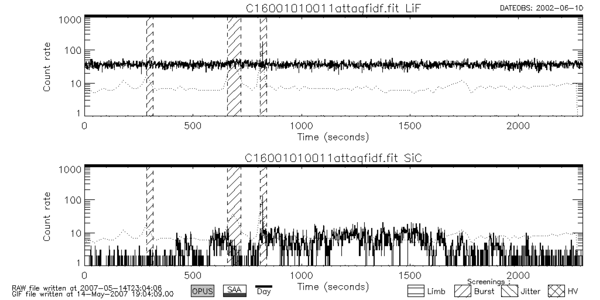 |
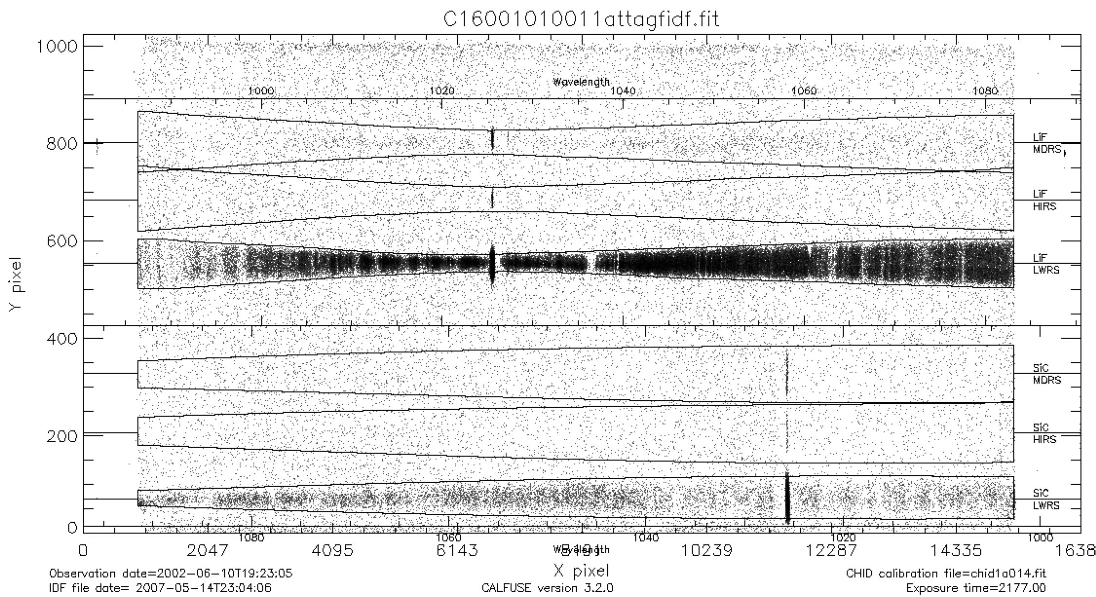
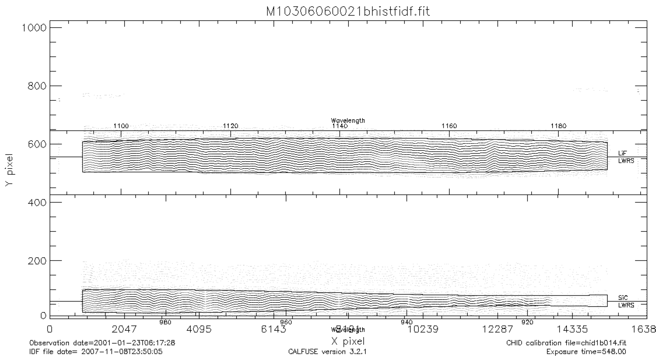
*ext.gif: These files show a calibrated image of the detector, corrected for geometric thermal distortions and spacecraft and instrumental motions. The appearance of these images depends on whether the exposure was TTAG or HIST observation (see Figs. 4.4 and 4.5). These plots only display the data from the "good time" intervals. Warning: if all of the data are flagged as bad, then, instead of producing an empty plot, all of the data are plotted. Therefore, users are recommended to systematicaly check the count rate plots first.
 |
 |
The trailer files contain run-time information for all pipeline modules. They also
list any warnings that these modules may have generated. The
"Intermediate" and "Advanced" users will want to look at the trailer files before using any data.
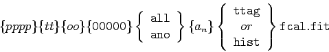
A trailer file is produced for each detector segment that is processed and its name
has the following form:
![\begin{displaymath}
\{ pppp \} \{ tt \} \{ oo \} \{ eee \}
\left\{ \begin{arra...
...]{c}{\tt ttag}\\ {\tt hist} \end{array} \right\}
{\tt f.trl}
\end{displaymath}](img86.png)
When rerunning CalFUSE, the content of the trailer file can be extended simply by changing the "verbose" level in
the CalFUSE parameter file. By default, the verbose level is set to 1. Table 4.13 gives
a short description of the verbose levels available to the users who
wish to rerun CalFUSE ("Advanced" level) along with corresponding examples of CalFUSE messages.
| Verbose Level: | 0 |
|---|---|
| Type | Minimal trailer file |
| Example | 2003 Mar 21 10:01:01 cf_ttag_init-1.12: WARNING - Detector voltage is high |
| Verbose Level: | 1 (Default) |
| Type | Standard trailer file |
| Messages | Lists all decisions made by the pipeline; Output from cf_timestamp when printing "Finished Execution"; Provides program/version information for other modules |
| Example | cf_timeline-1.1: Housekeeping file exists - use it to fill timeline. 2003 Mar 21 14:44:37 cf_timeline-1.1: Finished execution |
| Verbose Level: | 2 |
| Type | Verbose trailer file |
| Messages | Lists calls to cf_timestamp when printing "Begin execution" and "Finished execution" for all routines. Lists values calculated by the pipeline. Output from cf_timestamp has the Level 0 format; other entries are simply indented. |
| Example | 2003 Mar 21 14:44:37 cf_timeline-1.1: Begin execution State vector at MJD= 52577.192924 days x= 6712.928955 y= 106.584626 z= -2409.340612 km vx= 0.557736 vy= 7.210211 vz= 1.901099 km/s Number of samples in the HK file = 329 2003 Mar 21 14:44:37 cf_timeline-1.1: Finished execution |
| Verbose Level: | 3 |
| Type | Debugging mode |
| Messages | Lists milestones in each subroutine. Lists calibration files (especially when recorded elsewhere). |
| Example | Correcting y centroid Reading background calibration files Housekeeping file = M1070312001hskpf.fit Background calibration file = bkgd1a009.fit |
Note that verbose level N includes all information from level N—1 in addition to what is listed in
the Table. If a user chooses to rerun CalFUSE, occasional error and warning messages might appear in the
trailer files if a pipeline module fails to run successfully. Appendix C lists the warning messages
along with a short description of the problems likely to cause them. The error messages are self-explanatory.
Observation-level files combine all of the individual exposures for each
specific set of channel (LiF1, LiF2, SiC1 or SiC2) and segment (A, B). The
result is 8 independently obtained combined spectra with considerable wavelength
overlap. These overlapping regions provide redundancy in spectral coverage in order to
assess the consistency of the data and look for anomalies (see Chapter 7).
The two observation-level combined files are the ALL files, which contain
all of the data for a particular observation, and the ANO (All Night Only) files, which contain
only data obtained during orbital night. The former give the highest
signal-to-noise for instances where airglow is not an issue, and the latter
provide the best possible signal-to-noise with minimum airglow
contamination (see Chapter 7).
For each combination of detector segment and channel (LiF1A, SiC1A, etc.),
the pipeline combines data from all exposures constituting one observation into
separate extensions in a single ALL file. The combination results from cross-correlating and shifting the
individual exposures over the 1000-1100 Å overlap range. While the ALL files are well-suited for basic feature
searches, they are not optimized for science purposes. The "Intermediate" and "Advanced" users are
strongly advised to perform the spectral combinations carefully and as most appropriate to their science goals.
Each ALL file extension has 3 arrays: WAVE, FLUX and ERROR (see Table 4.14). For instance,
the first extention of the ALL file contains the combined LiF1A data for a given observation. For each
channel, the shift calculated for the detector segment spanning 1000-1100 Å is applied to the other
segment as well.
If the individual spectra are too faint for cross correlation, the individual Intermediate Data Files
(IDF) images are combined and a single spectrum is extracted from the combined IDFs (see Section 4.2.1.3).
The ANO files are identical to the ALL files, except that the spectra are
constructed using data obtained during the night-time portion of each
exposure only. They are generated only for TTAG data, and only if part of
the exposure occurs during orbital night. The shifts calculated for the
ALL files are applied to the ANO data and not recomputed. These data are essential to
identify airglow emission and to minimize their effect on overlapping stellar and/or
interstellar features (see Chapter 7).
The ALL and ANO file names have the following structure:
The first is the ALL file for LWRS (an = 4) , TTAG mode = ttag
data with for program pppp = D064, target number tt = 03,
observation ID oo = 01.
The second is an ANO file for MDRS aperture (an = 2),
TTAG (mode = ttag with program
pppp = E511, target number
tt = 22, observation ID
oo = 01.
NOTE: For dedicated airglow observations in programs M106 and S100, all
of the data are included
in the observation-level ALL, ANO, and NVO files (see below). For all other programs,
900-level airglow exposures are excluded from the sum. A single preview plot showing the summed
spectrum from all of the 900-level exposures
in the observation is produced with a name like M112580100000airgttagf.gif.
NOTE: The cataloging software used by MAST requires the presence of an ALL file for each exposure, in addition to the observation-level ALL file. Therefore, exposure-level ALL files are also generated, but they contain no data, only a FITS file header. The observation-level ALL files are distinguished by the string "00000all" in their names.
| FITS Extension | Format | Description |
|---|---|---|
| HDU 1: Empty (Header only)} | ||
| HDU 2: Mean LiF1A Extracted Spectrum (binary extension) | ||
| WAVE | FLOAT | Wavelength (Å) |
| FLUX | FLOAT | Flux (erg cm-2 s-1 Å-1) |
| ERROR | FLOAT | Gaussian error (\flux) |
| HDU 3: Same as HDU2 for mean LiF1B Spectrum} | ||
| HDU 4: Same as HDU2 for mean LiF2B Spectrum} | ||
| HDU 5: Same as HDU2 for mean LiF2A Spectrum} | ||
| HDU 6: Same as HDU2 for mean SiC1A Spectrum} | ||
| HDU 7: Same as HDU2 for mean SiC1B Spectrum} | ||
| HDU 8: Same as HDU2 for mean SiC2B Spectrum} | ||
| HDU 9: Same as HDU2 for mean SiC2A Spectrum} | ||
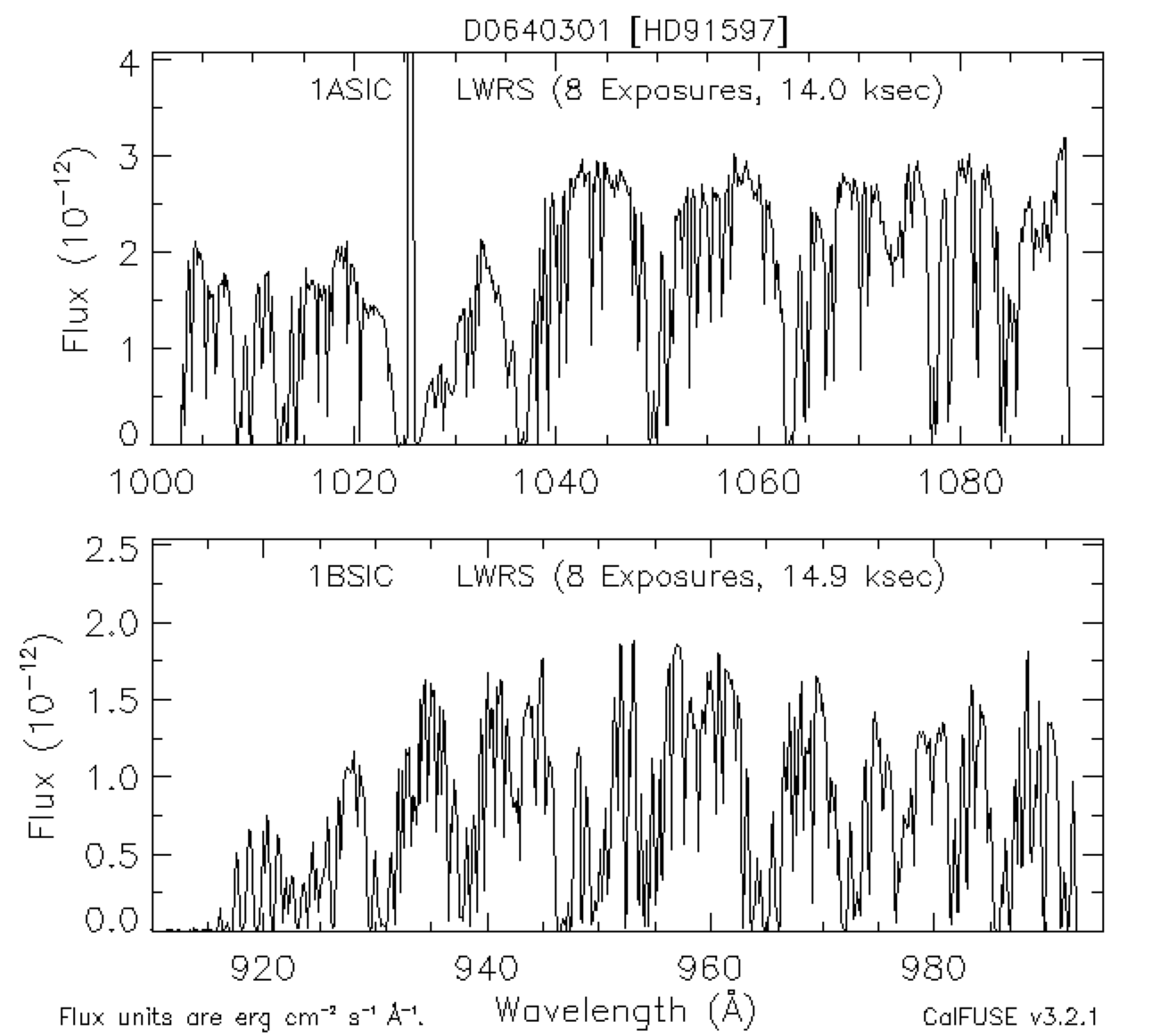
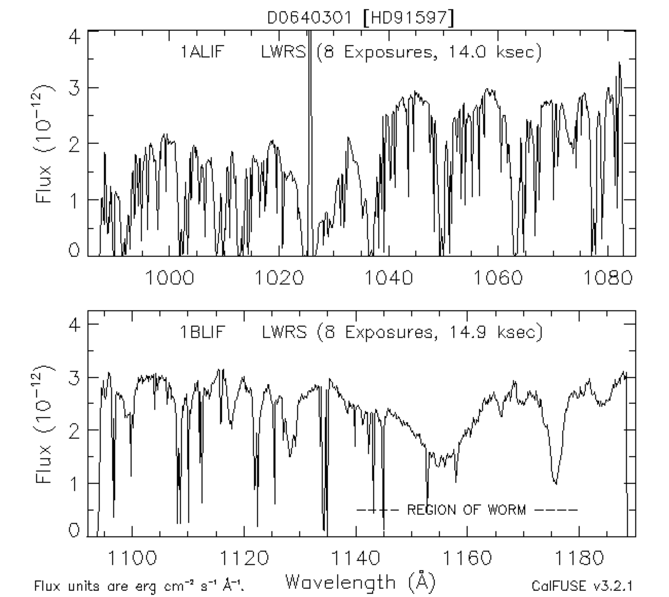
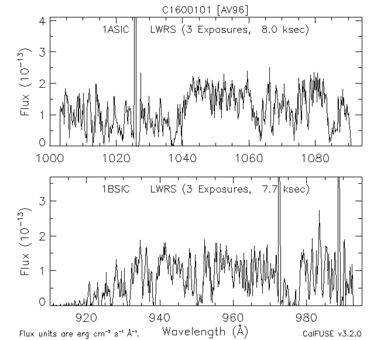
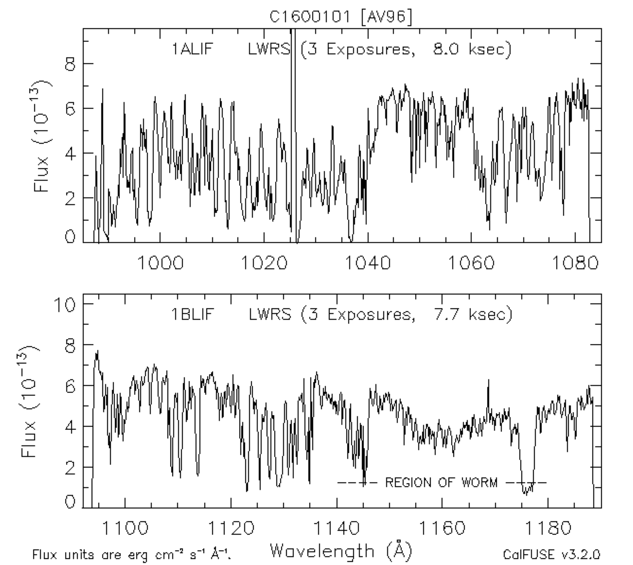
Coadded Detector Spectra (*00000*.gif)
The ALL files are used to generate a set of flux plots for the 4 channels
of each observation. These files have names of the type
D064030100000lif1ttagf.gif or D064030100000lif2ttagf.gif, etc.
Figures 4.6 and 4.7 show preview plots for the SiC1 (left) and LiF1 (right) channels of observations D0640301 and C1600101, respectively. Notice that even though the wavelength coverage of SiC1A and LiF1A have considerable overlap, they may have significantly different flux levels, as is the case for observation C1600101. Discrepancies of this type are common in FUSE data and usually indicate that the source was either partly or completely out of the aperture of one channel during part of the observation. Hence, the data obtained for the guiding channel are always the most reliable. With very few exceptions, LiF1 was the guiding channel before 12 July 2005, and LiF2 thereafter (see Table 2.3). These figures demonstrate the value of the diagnostic files for identifying systematic effects (see also Fig. 4.3 and
 |
|
 |
|
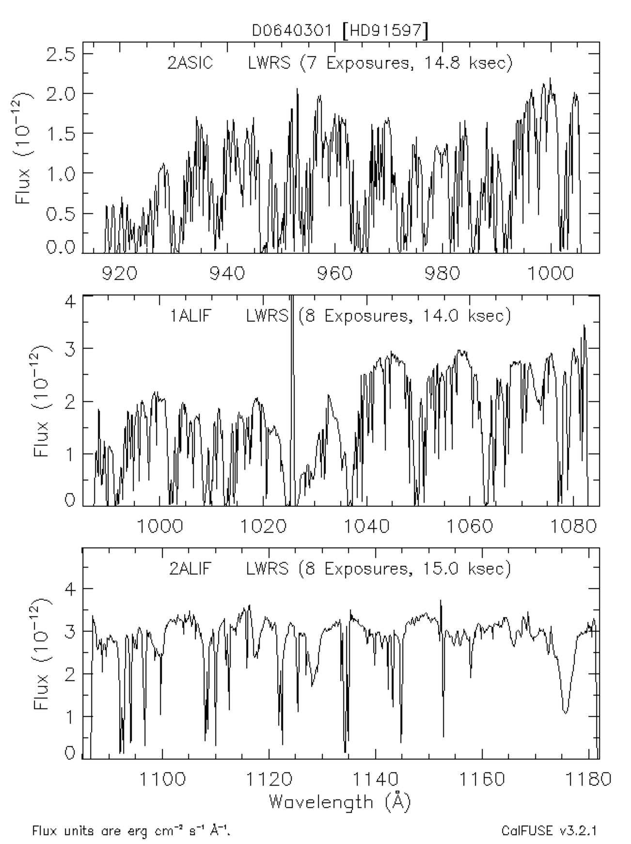
Preview Spectra (*spec*.gif)
These spectral plots are generated from the ALL files
for the channels exhibiting the highest S/N in the 900-1000, 1000-1100 and 1100-1200 Å regions
and thus offer a quick look at the entire FUSE wavelength range for a given observation.
These are the preview files presented by MAST when FUSE data are queried.
Figure 4.8 displays the preview file D064030100000specttagf.gif for observation D0640301.
 |
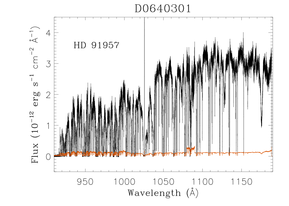
Summed Exposures (*nvo*.fit)
One National Virtual Observatory (NVO) file is generated for each
observation. This file contains one single spectrum spanning the entire
FUSE wavelength range (905 ≤ λ ≤ 1187Å). The spectrum is assembled by
cutting and pasting segments from the ALL file using the channel with the highest
signal-to-noise (S/N) ratio at each wavelength. Segments are shifted to match the guide channel
(either LiF1 or LiF2) between 1045 and 1070Å.
Warning: While these NVO spectra form a convenient overview of each data set, their direct
use for scientific analysis is not encouraged without detailed checking. Because of
possible channel drifts, the target may
have been outside of one or more apertures for some fraction of
the observation. Not only might the resulting spectrum
be non-photometric, but the photometric error may be wavelength-dependent, because of the way that the NVO
files are constructed. It is thus recommended that users examine the count-rate plots (see Section 4.2.1.4.)
for the individual exposures before accepting the NVO file at face value.
Additionally, cross-correlation may fail, even for the spectra of bright
objects, if they lack strong, narrow spectral features. Examples are nearby white
dwarfs with weak interstellar absorption lines. If cross-correlation fails
for a given exposure, that exposure is excluded from the sum. Thus, the
exposure time for a particular segment in an NVO file may be less than the
total exposure time actually available for a given observation.
NVO data files contain columns with WAVE, FLUX, and ERROR stored in a
single binary table extension (see Table 4.15).
Figure 4.9 shows the NVO spectrum of observation D0640301 for
target HD91597, with corresponding filename: D064030100000nvo4ttagfcal.fit.
 |
| FITS Extension | Format | Descriptions |
|---|---|---|
| HDU 1: Empty (Header only) | ||
| HDU 2: Extracted Spectrum (binary extension) | ||
| WAVE | FLOAT | Wavelength (Å) |
| FLUX | FLOAT | Flux (erg cm-2 s-1 Å-1) |
| ERROR | FLOAT | Gaussian error (erg cm-2 s-1 Å-1) |